
6. Regularity’s role in approximation#
We have already seen that the polynomial degree \(p\) and mesh size \(h\) are important factors in determining how best approximation errors of finite element spaces decrease. The regularity (or smoothness) of the approximating function also plays an important role. The purpose of this notebook is to illustrate the practical manifestation of the role of regularity in rates of approximation.
Here is a poem from the 1978 Finite Element Circus (a conference series on finite elements) that will reinforce the message.
There once was a fellow named Dare.
Who approximated PDEs with great care.
But the solutions were rough
And the problems were tough,
So he only got \(O(h^2).\)
In this notebook, we will see examples where we do not even get the \(O(h^2)\) approximation rate.
6.1. One-dimensional example#
Consider the function
on the interval \(0 < x < 1\). What is the rate of convergence of its best approximation in the lowest order DG finite element space built using a uniform mesh?
It is known from approximation theory that this convergence rate, for any given \(u\), is \(O(h)\) provided the derivative \(u'\) is in \(L_2(0,1)\) (and some other conditions hold). However, this result does not apply here since the derivative \(u'(x)\) of \(u(x) = x^{1/3}\) is not in \(L_2(0, 1)\). Since \(u \in L_2\) and \(u' \not\in L_2\), we suspect we might only get some intermediate convergence rate between 0 and 1 for the best approximation error of this \(u\). We proceed to compute this rate. Recall that the best approximation error is the error in the orthogonal projection and recall the following projection routine from a previous notebook.
import ngsolve as ng
import numpy as np
from ngsolve.meshes import Make1DMesh
from ngsolve import x, y, dx, sqrt, BilinearForm, LinearForm
from ngsolve.webgui import Draw
import matplotlib.pyplot as plt

def ProjectL2(u, W):
    """ Input: u as a CF.
        Output: L_2-projection Q u as a GF. """
    Qu = ng.GridFunction(W)
    q = W.TrialFunction()
    m = W.TestFunction()
    a = BilinearForm(q*m*dx)
    b = LinearForm(u*m*dx)
    with ng.TaskManager():
        a.Assemble()
        b.Assemble()
        Qu.vec.data = a.mat.Inverse(inverse='sparsecholesky') * b.vec
    return Qu
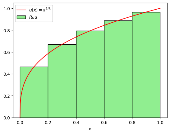
Here is a quick computation and visualization of the function \(u(x) = x^{1/3}\) and its \(L_2\)-orthogonal projection into the lowest order DG finite element space made with \(N\) elements, namely the function \((R_N u)(x)\) defined for \(x\) in each 1D element \( (x_i, x_{i+1})\) by
# Compute L_2 projection R_N on a uniform mesh of N elements
N = 5
mesh = Make1DMesh(5)
u = x**(1/3)
Ru = ProjectL2(u, ng.L2(mesh, order=0))
It is illustrative to visualize both \(u\) and \(R_N u\). Since these are functions of one variable, it makes sense to use matplotlib (rather than ngsolve) to plot them.
# Display u and R_N u
xv = np.array([v.point[0] for v in mesh.vertices])
xf = np.linspace(0, 1, 500)
uf = xf**(1/3)
fig, ax = plt.subplots()
exact, = ax.plot(xf, uf, 'r-')
proj = ax.bar(xv[:-1], Ru.vec, width=1/N, align='edge', fc='lightgreen', ec='k')
ax.set_xlabel('$x$')
ax.legend((exact, proj[0]), ('$u(x) = x^{1/3}$', '$R_N u$'));
To compute the rate of convergence of the best approximation, we again reuse the rate computation and tabulation routines from a previous notebook, with small modifications to suit this example.
def ProjectOnSuccessiveRefinements1D(u, p=0, N0=5, nrefinements=8):
    """Project to f.e. spaces on a sequence of uniformly refined meshes."""

    errors = []; N = N0
    for ref in range(nrefinements):
        mesh = Make1DMesh(N)
        W = ng.L2(mesh, order=p)
        Qu = ProjectL2(u, W)
        sqrerr = (Qu - u)**2
        errors.append(sqrt(ng.Integrate(sqrerr, mesh, order=max(2*p,10))))
        N *= 2
    return np.array(errors)

from prettytable import PrettyTable

def TabulateRate(name, dat, h0=1):
    """Inputs:
        name = Name for second (error norm) column,
        dat = list of error data on successive refinements
        log2h0inv = log2(1/h0), where h0 is coarsest meshsize.
    """
    col = ['h', name, 'rate']
    t = PrettyTable()
    h0col = ['%g'%h0]
    t.add_column(col[0], h0col + [h0col[0] + '/' + str(2**i)
                                  for i in range(1, len(dat))])
    t.add_column(col[1], ['%.8f'%e for e in dat])
    t.add_column(col[2], ['*'] + \
                 ['%1.2f' % r
                  for r in np.log(dat[:-1]/dat[1:])/np.log(2)])
    print(t)
es = ProjectOnSuccessiveRefinements1D(x**(1/3), N0=5, nrefinements=10)
TabulateRate('L2norm(Ru-u)', es, h0=1/5)
+---------+--------------+------+
|    h    | L2norm(Ru-u) | rate |
+---------+--------------+------+
|   0.2   |  0.05833905  |  *   |
|  0.2/2  |  0.03382494  | 0.79 |
|  0.2/4  |  0.01945306  | 0.80 |
|  0.2/8  |  0.01112239  | 0.81 |
|  0.2/16 |  0.00633195  | 0.81 |
|  0.2/32 |  0.00359315  | 0.82 |
|  0.2/64 |  0.00203399  | 0.82 |
| 0.2/128 |  0.00114923  | 0.82 |
| 0.2/256 |  0.00064839  | 0.83 |
| 0.2/512 |  0.00036541  | 0.83 |
+---------+--------------+------+
Clearly, the convergence rate of the lowest-order DG best approximation of \(u(x) = x^{1/3}\) appears to be
Question for discussion:
Through computations, can you guess how the above approximation rate (the convergence rate of the \(L_2\) best approximation from the \(p=0\) DG space) changes for \(u(x) = x^\gamma\) as you vary the power \(\gamma\)?
6.2. Two-dimensional example: the L-shape#
An L-shaped domain is a standard example in finite element analysis because it has a re-entrant corner that creates singularities in solutions of certain partial differential equations, even when the data is smooth. Here, we will use it to illustrate how the regularity of a function affects the convergence rate of its best approximation in a DG finite element space. Let \(\Omega = (-1, 1)^2 \setminus [0,1]\times [-1, 0]\) be the L-shaped domain shown below.
#
#  (-1,1)                       (1,1)
#       +----------------------+
#       |                      |
#       |                      |
#       |        (0,0)         |
#       |           +----------+ (1,0)
#       |           |
#       |           |
#       |           |
#       +-----------+
#  (-1,-1)       (0,-1)
#
We make this domain as an OpenCascade geometry object within netgen. It is put together below by combining three congruent squares into the inverted L-shape.
from netgen.occ import OCCGeometry, Rectangle, WorkPlane, Axes, X, Y, Z
from ngsolve.webgui import Draw

s1 = WorkPlane(Axes((0,0,0), n=Z, h=X)).Rectangle(1,1).Face()
s2 = WorkPlane(Axes((0,0,0), n=Z, h=-X)).Rectangle(1,1).Face()
s3 = WorkPlane(Axes((0,0,0), n=Z, h=Y)).Rectangle(1,1).Face()
L = s1+s2+s3
Draw(L);
geo = OCCGeometry(L, dim=2)
In this example, we are interested in computing the rate of convergence of the \(L_2(\Omega)\)-best approximation into the DG finite element space for the function
expressed in polar coordinates \(r, \theta\). As a first step, we want to visualize this function: it appears to have a fractional power behavior, similar to the previous 1D example, as one moves to the origin along a ray of constant polar angle. Let us define the polar coordinates as ngsolve coefficient functions.
from ngsolve import x, y, sin, cos, atan2
from math import pi

mesh = ng.Mesh(geo.GenerateMesh(maxh=1/8))
r = sqrt(x*x + y*y)
theta = atan2(y, x)
At this point, we should note that definining u = r**(2/3) * sin(2*theta/3) will not give the correct function! You will see the problem as soon as you plot the polar angle theta.
Draw(theta, mesh, 'theta');
As you can see, the branch cut in the definition of atan2 creates an unwanted discontinuity in \(\theta\) right through our domain \(\Omega\). We want \(\theta\) to be a continuous function in \(\Omega\) because otherwise functions with fractional angle dependence, like \(\sin(2 \theta/3)\) would exhibit spurious discontinuities that should not exist, e.g., if you ask to Draw(sin(2*theta/3), mesh) you will see the problem in the output.
A simple solution is to rotate the coordinate system, take arctan, and then rotate the result back. This essentially puts the branch cut outside our domain’s interior. Below, we implement this idea using the rotation matrix
with \(\alpha = -3\pi/4\).
alpha = -(pi/2 + pi/4)
rotatedx = ng.cos(alpha) * x - ng.sin(alpha) * y
rotatedy = ng.sin(alpha) * x + ng.cos(alpha) * y
theta = ng.atan2(rotatedy, rotatedx) - alpha
Draw(theta, mesh, 'theta');
With this revised theta, we can now visualize \(u = r^{2/3}\sin(2\theta/3).\) Note that \(u\) is smooth at all points away from the so-called re-entrant corner, the corner vertex at which the domain’s edges subtend an obtuse angle within the domain.
u = r**(2/3) * ng.sin(2*theta/3)
Draw(u, mesh);
To compute the best approximation rates, as before, we use a sequence of meshes obtained by successive uniform refinement.
def ProjectOnSuccessiveRefinements2D(u, p=1, hcoarse=1, nrefinements=8):
    """Project to f.e. spaces on a sequence of uniformly refined meshes."""

    errors = [];
    mesh = ng.Mesh(geo.GenerateMesh(maxh=hcoarse))
    for ref in range(nrefinements):
        W = ng.L2(mesh, order=p)
        Qu = ProjectL2(u, W)
        sqrerr = (Qu - u)**2
        errors.append(sqrt(ng.Integrate(sqrerr, mesh)))
        mesh.ngmesh.Refine()
    return np.array(errors)
es = ProjectOnSuccessiveRefinements2D(u, p=1, nrefinements=8)
TabulateRate('L2norm(Qu-u)', es)
+-------+--------------+------+
|   h   | L2norm(Qu-u) | rate |
+-------+--------------+------+
|   1   |  0.05265536  |  *   |
|  1/2  |  0.01845368  | 1.51 |
|  1/4  |  0.00617248  | 1.58 |
|  1/8  |  0.00201338  | 1.62 |
|  1/16 |  0.00064758  | 1.64 |
|  1/32 |  0.00020659  | 1.65 |
|  1/64 |  0.00006559  | 1.66 |
| 1/128 |  0.00002076  | 1.66 |
+-------+--------------+------+
We observe a convergence rate of about \(O(h^{1 + 2/3})\), clearly falling short of \(O(h^2)\).
Questions for discussion:
How does the above observed rate change as \(p\) changes?
What if you measure the error in the \(H^1\) norm instead of the \(L_2\) norm? How does the rate change with \(p\) in that case?
Repeat the convergence rate study for the function
\[ u = r^2 \sin(2\theta/3). \]The higher power of \(r\) makes it smoother than the previous case, so we expect faster rates. Report how these rates change with the polynomial degree \(p\).
How would you quantify the difference in the regularity of \(u = r^{2/3} \sin(2\theta/3)\) and \(u = r^2 \sin(2\theta/3)\)?
6.3. Summary#
We have seen
that the regularity of a function limits its best approximation rates,
that singularities even at one boundary point can reduce rates in 2D,
the often-used L-shaped domain, and so-called re-entrant corners,
limited rates of best approximation of functions with fractional powers in 1D,
a branch cut creating spurious discontinuities in polar coordinates, and
that increasing the polynomial degree may have limited benefits when the approximated function has low regularity.