7. The confusion problem#
The stationary convection-diffusion problem treated using the standard finite element method can produce unstable solutions, a notorious issue often colloquially referred to as the Con-fusion Problem. In this notebook, we see how these instabilities emerge. This will serve as motivation for further studies into other finite element extensions more appropriate for treating convection-diffusion problems.
Many practically interesting scientific models feature both diffusion and convection. Heat flow is a typical example. Fourier’s law of heat conduction states that heat flux \(q_{\text{conductive}}\) is proportional to the negative temperature gradient: \(q_{\text{conductive}} = - \kappa \grad u\), where \(u\) denotes the temperature and the constant of proportionality, \(\kappa\), is called the thermal conductivity. Convective heat flux takes the form \(q_{\text{convective}} = \beta u\) where \(\beta\) is an advection velocity vector field that transports heat along it. By conservation of energy the heat lost through the sum of these fluxes on any control volume \(V\) must equal the sum of heat sources \(f\) within it:
where \(n\) denotes the outward unit normal. Transforming this integral law into a differential one as usual, we obtain the convection-diffusion equation,
which one might also rewrite as
in the often-occurring case of \(\div \beta=0\). There is nothing confusing about finite element application for this equation when \(\kappa\) and \(\beta\) are nice. Confusion might arise when \(\beta\) is too large, or when \(\kappa\) is too small, cases where the standard Lagrange finite element method can give strange solutions, as seen below.
7.1. A model problem#
A simple model boundary value problem with the convection-diffusion equation is as follows.
where \(n\) is the outward unit normal. To obtain a nice test problem we choose very smooth data (so that no tricks are needed to integrate the data accurately), namely
and assume that \(\kappa>0\) is a constant function.
Questions for discussion:
For the specific data above, would the solution depend on both \(x\) and \(y\)?
What happens if you plug in the following expression into the PDE and boundary conditions?
7.2. Finite element solution#
The weak formulation is derived as usual by multiplying by a test function \(v\) and integrating by parts. Namely, letting \(\Gamma\) be the subset of \(\partial\Omega\) consisting of the left and right boundary segments with Dirichlet data, the weak solution \(u\) satisfies
for all test functions \(v\) (in the appropriate space) that vanish on \(\Gamma\). To treat the non-homogeneous Dirichlet boundary conditions, as usual, we let \(u_g\) be an extension into \(\Omega\) of the boundary data \(g\). Then writing
we find the function \(\mathring u\) with zero boundary conditions on \(\Gamma\) by solving \( b(\mathring u, v) = \ell(v) - b(u_g, v) \) for all \(v\) in the space space and \(\mathring u\).
We proceed to solve the Galerkin approximation of this problem using Lagrange finite elements of degree \(p \ge 1\). More precisely, letting \(\mathring{V}^{\Gamma}_{hp}\) denote the subspace of the degree \(p\) Lagrange finite element space of functions that vanish on \(\Gamma\), we solve for \(\mathring u_h\) in \(\mathring{V}^{\Gamma}_{hp}\) satisfying
for all \(v_h\) in \(\mathring{V}^{\Gamma}_{hp}\), and then set \(u_h = \mathring u_h + u_g\). This process is implemented in the following code using NGSolve.
import ngsolve as ng
import numpy as np
from ngsolve.webgui import Draw
from netgen.geom2d import unit_square
from ngsolve import grad, dx, ds, CoefficientFunction, GridFunction, BilinearForm, LinearForm
from ngsolve.solvers import GMRes
# Set convection veclocity

beta = CoefficientFunction((1, 0))

# Set Gamma = left|right and space with essential b.c.

mesh = ng.Mesh(unit_square.GenerateMesh(maxh=0.1))
V = ng.H1(mesh, order=2, dirichlet='left|right')

# Inhomogeneous Dirichlet b.c.

g = 0.5
def SolveConfusion(mesh, kappa=1, p=2):
    """Use Lagrange finite elements to approximate the above
    variational formulation of the confusion model problem."""

    V = ng.H1(mesh, order=p, dirichlet='left|right')
    u, v = V.TnT()

    a = BilinearForm(V)
    a+= (kappa*grad(u)*grad(v) - u*beta*grad(v)) * dx
    c = ng.Preconditioner(a, "local") # used only for gmres
    f = LinearForm(V)
    uh = GridFunction(V)

    with ng.TaskManager():
        # Assemble
        uh.Set(g, definedon=mesh.Boundaries('left'))
        a.Assemble()
        f.Assemble()

        # Solve
        f.vec.data -= a.mat * uh.vec

        try: # use direct nonsymmetric sparse solver if available

            uh.vec.data += a.mat.Inverse(freedofs=V.FreeDofs(), inverse='umfpack') * f.vec

        except:  # if not, use iterative solver gmres
            u0 = uh.vec.CreateVector(); u0[:] = 0
            GMRes(A=a.mat, pre=c, b=f.vec, x=u0, tol=1e-15, printrates=False, maxsteps=1000)
            uh.vec.data += u0

    return uh
uh = SolveConfusion(mesh, kappa=0.3, p=3)
Draw(uh, deformation=True,
     settings={"camera" : {"transformations" :[{"type": "rotateX", "angle": -30},{"type": "rotateY", "angle": -10},{"type": "rotateZ", "angle": -10}]}});
To compare this with the exact solution, recalling from above discussion that the exact solution has no \(y\) dependence, we may plot the exact solution as one-variable function of \(x\) and compare it with the above multidimensional plot.
import numpy as np
import matplotlib.pyplot as plt
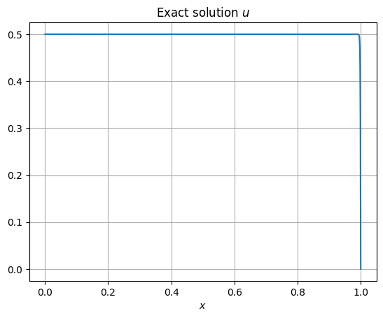
def plotexact(kappa):
x = np.linspace(0, 1, 1000)
u = (1 - np.exp((x-1)/kappa)) / (1-np.exp(-1/kappa)) / 2
plt.plot(x, u); plt.xlabel('$x$'); plt.grid(True); plt.title('Exact solution $u$')
plotexact(kappa=0.3)
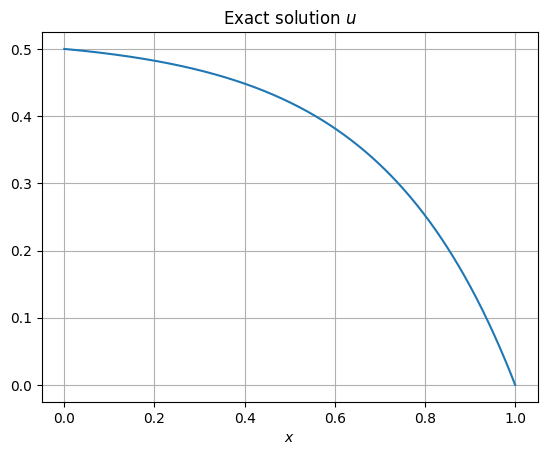
Clearly, the exact solution and the discrete solution looks visually identical. Of course, to get definitive verification, we must compute the errors and its convergence rates, which is left as an exercise.
Questions for discussion:
To get definitive verification that the computed solution is close to the above exact solution, we must compute the errors and its convergence rates. How would you do this?
As an example, fix \(\kappa = 1/3\), what does your computations predict regarding the of convergence of \(\| u - u_h \|_{L^2(\Omega)}\) and \(\| u - u_h \|_{H^1(\Omega)}\) as \(h\) tends to 0?
7.3. What happens to the discrete solution as \(\kappa \to 0\)?#
The reason for studying this con-fusion problem is to understand when and why we do not get nice solutions from the finite element method. To this end, we compute solutions for smaller and smaller \(\kappa\) while comparing the exact and discrete solutions for each \(\kappa\) value.
7.3.1. Case of \(\kappa = 1/10\)#
plotexact(kappa=0.1)
uh = SolveConfusion(mesh, kappa=0.1, p=3)
Draw(uh, deformation=True,
     settings={"camera" : {"transformations" :[{"type": "rotateX", "angle": -30},{"type": "rotateY", "angle": -10},{"type": "rotateZ", "angle": -10}]}});
The discrete solution continues to match the exact solution quite nicely when \(\kappa=0.1\). How about when \(\kappa\) is reduced by a factor of 10?
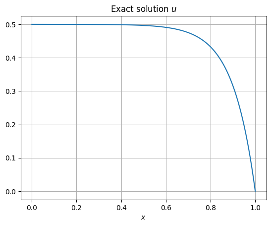
7.3.2. Case of \(\kappa = 1/100\)#
plotexact(kappa=0.01)
uh = SolveConfusion(mesh, kappa=0.01, p=3)
Draw(uh, deformation=True,
     settings={"camera" : {"transformations" :[{"type": "rotateX", "angle": -30},{"type": "rotateY", "angle": -10},{"type": "rotateZ", "angle": -10}]}});
Note the emergence of overshoots at the boundary layer of the exact solution. We see that the method is having difficulties capturing the sharp transition there. What if we reduce \(\kappa\) by another factor of 10?
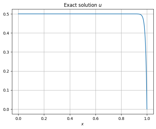
7.3.3. Case of \(\kappa = 1/1000\)#
plotexact(kappa=0.001)
uh = SolveConfusion(mesh, kappa=0.001, p=3)
Draw(uh, deformation=True,
     settings={"camera" : {"transformations" :[{"type": "rotateX", "angle": -30},{"type": "rotateY", "angle": -10},{"type": "rotateZ", "angle": -10}]}});
The discrete solution appears to have become useless.
These observations illustrate that as diffusion vanishes (i.e., as \(\kappa \to 0\)), the numerical solutions may not look anything like the exact solution and has spurious oscillations. Note that as \(\kappa\) becomes smaller, the exact solution has an increasingly thin boundary layer.
Of course, we should expect any method to have difficulties capturing the sharp transition in such thin boundary layers. What is troublesome in the above observations is that tolerable oscillations emanating from a thin boundary layer has spread out over the whole domain and destroyed the solution even in locations far away from the boundary layer. This is a telltale sign of an unstable method.
Question for discussion:
Why does the theory not rule out this instability?
7.4. Stationary advection equation#
After having examined the small \(\kappa\) cases above, it is natural to ask what happens if \(\kappa=0\)? When \(\kappa=0\), we obtain the (stationary) convection equation, also known as stationary advection equation, modeling pure transport without any diffusion. Continuing to assume that the convection vector field \(\beta\) satsifies \(\div \beta = 0\), the partial differential equation obtained when \(\kappa=0\) is
This first-order equation cannot admit boundary conditions on the entire boundary. One can see using characteristics that this partial differential equation admits boundary values on the inflow boundary defined by
On the outflow boundary \(\partial_{out} \Omega = \{ x \in \partial\Omega:\; b \cdot n >0\}\) and on the remainder \(\partial \Omega \setminus (\partial_{in} \Omega \cup \partial_{out} \Omega)\), no boundary conditions should be placed. Thus, the stationary advection boundary value problem we shall consider is to solve for u satisfying
As in the convection-diffusion case, we consider simple data of the form
Then \(\partial_{in} \Omega \) is the left boundary segment of the unit square domain. Moreover, the exact solution is simply \(u \equiv 1/2\) on the entire domain \(\Omega\).
We proceed to see two finite element methods for this case. The first one is a natural extension of what we have already seen for the convection-diffusion equation.
7.4.1. A tempting limit method#
Recall that the method for the convection-diffusion case finds \(u_h\) in \(u_g + \mathring{V}^{\Gamma}_{hp}\) satisfying
for all \(v_h \in \mathring{V}^{\Gamma}_{hp}\).
Succumbing to the temptation of just putting \(\kappa=0\) in this equation to get a method for the advection equation (and resetting \(\Gamma\) in \(\mathring{V}^{\Gamma}_{hp}\) to consist only of the inflow boundary), we construct the following implementation by a minor modification of the previous convection-diffusion code (the modifications being the elimination of the \(\kappa\) term and the change of the dirichlet flag to left). The implemented method finds \(u_h \in u_g + \mathring{V}^{\Gamma}_{hp}\), where \(\Gamma\) now consists only of the inflow boundary, satisfying
for all \(v_h \in \mathring{V}^{\Gamma}_{hp}\).
def SolveConv(mesh, p=2):
    """Solve advection equation by minimal modification of the
    previous convection-diffusion code for zero diffusion."""

    V = ng.H1(mesh, order=p, dirichlet='left')
    u, v = V.TnT()

    a = ng.BilinearForm(V)
    a+= -u*beta*grad(v) * dx
    c = ng.IdentityMatrix(size=V.ndof)
    f = ng.LinearForm(V)
    uh = ng.GridFunction(V, 'u_strongBC')

    with ng.TaskManager():
        uh.Set(1, definedon=mesh.Boundaries('left'))
        a.Assemble()
        f.Assemble()

        f.vec.data -= a.mat * uh.vec
        try:
          uh.vec.data += a.mat.Inverse(freedofs=V.FreeDofs(), inverse='umfpack') * f.vec
        except:
          u0 = uh.vec.CreateVector(); u0[:] = 0
          GMRes(A=a.mat, pre=c, b=f.vec, x=u0, tol=1e-10, printrates=False, maxsteps=10000)
          uh.vec.data += u0

    return uh
Unfortunately, this method does not work.
uh = SolveConv(mesh, p=3)
Draw(uh, deformation=True,
     settings={"camera" : {"transformations" :[{"type": "rotateX", "angle": -30},{"type": "rotateY", "angle": -10},{"type": "rotateZ", "angle": -10}]}});
Clearly, the same problem from the convection-diffusion case persists, and has even gotten worse. This shows that blindly taking the singular limit \(\kappa=0\) in a variational formulation is problematic.
Question for discussion:
How does this compare with an alternative method described next? Setting \(\Gamma\) to the inflow boundary, this method also uses \(\mathring{V}^{\Gamma}_{hp}\), but solves for \(u_h \in u_g + \mathring{V}^{\Gamma}_{hp}\) satisfying
\[ \int_\Omega (\beta \cdot\grad u_h ) v_h = \int_\Omega f v_h \]for all \(v_h \in \mathring{V}^{\Gamma}_{hp}\).
7.4.2. Lagrange finite elements with weakly imposed inflow boundary condition#
An alternate approach is motivated by the following computational thinking. At the singular limit of \(\kappa=0\), the essential boundary conditions suddenly change (and so does the space in the weak form). Could we formulate a weak form where one could use the same space for \(\kappa>0\) and for \(\kappa=0\)? Also, reviewing the solutions computed for the convection-diffusion equation, it appears as if our method is overly constrained by the need to satisfy the boundary conditions strongly, or exactly. Could we relax the imposition of the boundary condition in some way?
These questions are answered by a simple technique of weak imposition of boundary condition. To explain this, let us start from
and develop an alternate weak formulation: multiply by a test function \(v\) (without any boundary condition) and integrate by parts. Then we seek \(u \in H^1(\Omega)\) satisfying
for all \(v \in H^1(\Omega).\) Note that the inflow boundary condition is no longer imposed essentially in the space, rather it is incorporated into the equation while integrating by parts in a natural fashion. This technique of boundary condition imposition is called weakly imposed inflow boundary condition.
It is straightforward to implement a Lagrange finite element approximation based on this new weak form, as seen below.
def SolveConvectionWeakBC(mesh, p=2):
    """Same as the above code for convection-diffusion,
    but now with no diffusion"""

    V = ng.H1(mesh, order=p) # No boundary condition in V !
    u, v = V.TnT()
    n = ng.specialcf.normal(2)

    a = ng.BilinearForm(V)
    a+= -u*beta*grad(v) * dx
    a+= beta*n * u * v * ds(definedon='right')
    c = ng.IdentityMatrix(size=V.ndof)
    f = ng.LinearForm(V)
    f+= -beta * n * g * v * ds(definedon='left')

    uh = ng.GridFunction(V, 'u_weakBC')

    with ng.TaskManager():
        uh.Set(1, definedon=mesh.Boundaries('left'))
        a.Assemble()
        f.Assemble()

        f.vec.data -= a.mat * uh.vec

        try:
          uh.vec.data += a.mat.Inverse(freedofs=V.FreeDofs(), inverse='umfpack') * f.vec
        except:
          u0 = uh.vec.CreateVector(); u0[:] = 0
          GMRes(A=a.mat, pre=c, b=f.vec, x=u0, tol=1e-10, printrates=False, maxsteps=10000)
          uh.vec.data += u0

    return uh
With this way of imposing boundary conditions, we obtain good results.
uh = SolveConvectionWeakBC(mesh, p=3)
Draw(uh, deformation=True, autoscale=False, min=0, max=.5,
     settings={"camera" : {"transformations" :[{"type": "rotateX", "angle": -30},{"type": "rotateY", "angle": -10},{"type": "rotateZ", "angle": -10}]}});
The computed solution is visually indistinguishable from the exact solution \(u \equiv 1/2\). We have demostrated that there does seem to be an advantage in imposing the boundary conditions weakly, at least for this simple advection example.
These experiments here have set the stage for study of better methods for convection-dominated problems. Later, we shall study Discontinuous Galerkin (DG) finite element methods which remain stable in the convection-dominated regime as well as in the pure advection case. The DG method can be viewed as a method obtained by applying the idea of weak boundary condition imposition not just on the boundary of the domain, but to the boundary of every element in the mesh. As we shall see, they lead to practically useful methods with rigorously provable stability properties.
7.5. Summary#
We have made these observations in this notebook:
The standard finite element method for the convection-diffusion equation appears to work well when diffusion is of unit order and convection is moderate.
However, the same method can produce unstable solutions when convection dominates diffusion.
As diffusion vanishes, the numerical solutions may exhibit spurious oscillations that spread throughout the domain, indicating instability.
The pure advection case cannot be treated satisfactorily by blindly setting the diffusion to zero in the method.
Weakly imposing boundary conditions can help stabilize the method in the pure advection case.