
3. Convergence rates#
Convergent quantities, such as errors in numerical approximations of functions, often decrease to zero with respect to some approximation space parameters. Being able to compute the rate of convergence of such quantities is important in computational experimentation.
In a prior activity, we computed the \(L_2\) best approximation of some given function \(u\) from a finite element space \(S_h\). Given a function \(\newcommand{\om}{\varOmega}\) \(u \in L_2(\om)\), its Best Approximation Error from a finite element subspace \(S_h\) of \(L_2(\om)\) is
In this notebook, we are interested in quantifying how this BAE becomes small as the mesh size \(h\) (the maximal diameter \(h\) of all mesh elements) is decreased and as the polynomial degree \(p\) increases. This is done by computing rates of observed convergence. To fix a finite element space, we set \(S_h\) to \(W_{hp}\) throughout: recall that it is the “DG space” \( W_{hp} = \{ w: w|_K\) is a polynomial of degree \(\le p\) on each mesh element \(K\}.\)
3.1. Orthogonal projections#
We saw that the best approximations can be computed by minimizing a nonlinear distance functional in a previous notebook. In exercises, we have also seen that the minimizer equals the \(L_2\)-orthogonal projection onto the finite element space. Let \(\newcommand{\om}{\varOmega}\) \(Q_{hp}: L_2(\om) \to W_{hp}\) denote the \(L_2\)-orthogonal projection onto \(W_{hp}\). The norm and the inner product in \(L_2(\om)\) are, respectively, defined by
We will use the following two properties left as exercises:
Property 1. The \(L_2\)-projection \(Q_{hp} u\) is the best approximation to a \(\newcommand{\om}{\varOmega}\) \(u \in L_2(\om)\) from the subspace \(M\), namely,
Property 2. \(Q_{hp} u\) satisfies \(\newcommand{\om}{\varOmega}\)
and any \(u \in L_2(\om)\).
The right hand side of equation (1) equals the BAE\((u)\) of \(u\) from \(W_{hp}\). Thus Property 1 implies that we can compute BAE\((u)\) if we can compute \(Q_{hp} u\) and the norm of the difference \(\| u - Q_{hp} u \|_{L_2(\om)}\).
3.2. Computing the \(L_2\)-orthogonal projection#
Property 2 gives us a way to compute the \(L_2\)-orthogonal projection by solving a linear system, as we shall see below. Property 1 then tells us that we have in fact computed the best approximation. Therefore this gives us an alternate linear method, (at least superficially) distinct from the nonlinear method of a prior notebook, to compute best approximations.
Namely, given a \(u \in L_2(\om)\), by (2), its best approximation from \(W_{hp}\) is the function \(q = Q_{hp} u\) in \(W_{hp}\) satisfying
We will encounter many more equations of this type in this course, so it pays to delve into a bit more detail. All such equations will be of the form
and they are often called equations of forms or variational equations.
For the projection computation, \(a(\cdot,\cdot)\) is the just the inner product \((\cdot, \cdot)_{L_2(\om)}\), while \(b(\cdot)\) equals \((u, \cdot)_{L_2(\om)}\).
Let us get acquainted with some terminology related to equations like \(a(q, w) = b(w)\) right away:
The set of functions from which the solution \(q\) is to be found is called the set of trial functions.
The set of functions \(m\) for which the equation must hold is called the set of test functions. (In the projection example, the spaces of trial and test functions are the same, but they need not always be so.)
The right hand side is called a linear form since it is linear in the test function \(w\). (In the projection example, it contains the problem data involving the given function \(u\).)
The left hand side is called a bilinear form (since it is linear in both the trial function \(q\) and the test function \(w\)).
You will see these names being used for the corresponding ngsolve objects below.
import ngsolve as ng
from netgen.occ import unit_square
from ngsolve import dx, x, y, sin, BilinearForm, LinearForm, Mesh

def ProjectL2(u, W):
    """ Input: u as a CF.
        Output: L_2-projection Q u as a GF. """
    Qu = ng.GridFunction(W)
    q = W.TrialFunction()  # Alternate one-liner:
    w = W.TestFunction()   #   q, w = W.TnT()
    A = BilinearForm(q*w*dx)
    B = LinearForm(u*w*dx)

    with ng.TaskManager():
        A.Assemble()
        B.Assemble()
        Qu.vec.data = A.mat.Inverse(inverse='sparsecholesky') * B.vec
    return Qu
Before explaining the code, let us visualize a smooth function and its projection into the space of piecewise constant functions.
from ngsolve.webgui import Draw

h = 0.2
mesh = ng.Mesh(unit_square.GenerateMesh(maxh=h))
p = 0    # the piecewise constant DG space
Whp = ng.L2(mesh, order=p)

u = sin(5 * x * y)
Qu = ProjectL2(u, Whp)

Draw(u, mesh); Draw(Qu);
3.3. Conversion to a matrix problem#
In the code above, notice the Assemble and Inverse methods. The first converts equations of forms
in a generic space \(W\), represented as W in the computations, into a matrix system, using a basis for W, as explained next.
Suppose \(\Theta_1, \ldots, \Theta_N\) form a set of global shape functions of the finite element space W. (We have talked about global shape functions both in 1D and in 2D for several finite element spaces in prior notebooks.) Then expanding the unknown function \(q \in W\) in the basis of global shape functions,
we find that, with \(w=\Theta_i\), the equation (3) imply
for every \(i=1, \ldots, N\). Hence, defining a matrix \(A \in \mathbb{R}^{N \times N}\) and a vector \(B \in \mathbb{R}^N\) by
we have converted the problem of finding \(q \in W\) into a problem of finding a vector \(X \in \mathbb{R}^N\) satisfying
This is the process that happens behind the scenes when the Assemble method is called. In the code for the function ProjectL2, the object a.mat contains the matrix \(A\) (in a sparse format) and b.vec contains the vector \(B\) after the Assemble methods are completed. Matrices \(A\) generated in this way from a bilinear form \(a(\cdot, \cdot)\) are called stiffness matrices of the form \(a\).
To compute the vector \(X\),
we use the line in the code where A.mat.Inverse(...) is multiplied by B.vec. Knowing the vector \(X\) is the same as knowing everything about the function \(q\) due to (4).
The inverse='sparsecholesky' keyword within the Inverse method calls an ngsolve implementation of a version of Cholesky factorization for sparse matrices. It only works for symmetric/Hermitian and positive definite matrices. (Is the matrix for the projection problem such a matrix?) For more general sparse matrices, it is advisable to use a professional sparse matrix solver such as umfpack, pardiso, or mumps. A standard installation of ngsolve usually contains one of them, set to the default that is called when you do not specify a value for the inverse keyword argument. (To see which one you have, try setting inverse='umfpack' or inverse='pardiso' and see which one works.)
3.4. Successive mesh refinements#
We now proceed to study the best approximation error over a collection of meshes whose element shapes do not vary over the collection, even if their element sizes might vary considerably. A sequence of increasingly finer meshes where the element angles never change from those of the coarsest mesh is obtained by a simple uniform refinement. This is illustrated in the sequence of mesh images below.
mesh = Mesh(unit_square.GenerateMesh(maxh=0.3))
Draw(mesh);
mesh.ngmesh.Refine(); Draw(mesh);
mesh.ngmesh.Refine(); Draw(mesh);
Clearly this process of uniform refinement, when started on any coarse mesh, does not generate any new angles within the new elements, i.e., each triangular element of this infinite sequence of meshes is similar (in the geometric sense) to one of the triangles in the initial coarse mesh.
3.5. Projections on uniform refinements#
Next, we compute the \(L_2\) projection on a sequence of uniform refinements, starting from a very coarse mesh, using the function below. We then compute the \(L_2\)-norm of the error \(\| u - Q_{hp} u\|_{L_2(\om)}\) using the Integrate method provided by ngsolve.
from ngsolve import Integrate, sqrt
import numpy as np

def ProjectOnSuccessiveRefinements(u, p=0, hcoarse=1, nrefinements=8):
    """Project to f.e. spaces on a sequence of uniformly refined meshes."""

    Qus = []; errors = []; meshes = []; ndofs = []
    mesh = ng.Mesh(unit_square.GenerateMesh(maxh=hcoarse))

    for ref in range(nrefinements):
        W = ng.L2(mesh, order=p)
        Qu = ProjectL2(u, W)
        sqrerr = (Qu - u)**2

        Qus.append(Qu)
        errors.append(sqrt(Integrate(sqrerr, mesh)))
        meshes.append(ng.Mesh(mesh.ngmesh.Copy()))
        ndofs.append(W.ndof)

        mesh.ngmesh.Refine()

    return Qus, np.array(errors), ndofs, meshes
We select an infinitely smooth function \(u\) for the initial experiments (and you can experiment with less regular functions in exercises). Additionally, let us ensure that the smooth \(u\) has some mild oscillations (as otherwise the approximation errors reduce very rapidly and become too close to machine precision and rate computation becomes unreliable).
u = sin(5*x*y)
Qus, es, ns, _ = ProjectOnSuccessiveRefinements(u, p=0)
errors = {0: es}; ndofs = {0: ns}
es  # display the sequence of error norms just computed
array([0.61147848, 0.3888668 , 0.19805796, 0.09974437, 0.04996571,
       0.02499467, 0.01249882, 0.00624959])
Observe that this sequence of error norms are decreasing, approximately halving at each step. This immediately gives us an indication of the expected rate of convergence of the error: indeed, any quantity that decreases to zero like \(O(h)\) will halve each time the mesh size \(h\) is halved. (In contrast, a quantity that decreases like \(O(h^2)\) will quarter each time \(h\) is halved.) Anticipating more general error sequences in other cases, let us get organized for systematic rate computations.
3.6. Estimate rate of convergence#
We want to estimate at what rate the errors on successive refinements (stored in the above list es) go to zero. Let \(e_i\) denote the \(i\)th element of the list.
Specifically, what we would like to determine is the number \(r\), the rate of convergence, such that the errors are bounded by \(O(h^r).\) If the sequence \(e_i\) goes to zero like \(O(h_i^r)\), then since the refinement pattern dictates
we should see \(e_{i+1} / e_i \sim O(2^{-r})\). Hence to estimate \(r\), we compute
These logarithms are computed and tabulated together with the error numbers using the formatting function below. For formatting, we use a small external library called prettytable.
from prettytable import PrettyTable

def TabulateRate(name, dat, h0=1):
    """Inputs:
        name = Name for second (error norm) column,
        dat = list of error data on successive refinements,
        h0 = coarsest meshsize.
    """
    col = ['h', name, 'rate']
    t = PrettyTable()
    h0col = ['%g'%h0]
    t.add_column(col[0], h0col + [h0col[0] + '/' + str(2**i)
                                  for i in range(1, len(dat))])
    t.add_column(col[1], ['%.12f'%e for e in dat])
    t.add_column(col[2], ['*'] + \
                 ['%1.2f' % r
                  for r in np.log(dat[:-1]/dat[1:])/np.log(2)])
    print(t)
Next, we will apply this function to tabulate rates of convergence for each \(p\) using a series of uniformly refined meshes. Both the error norms and the rate computed using the log-technique are tabulated for each degree considered.
3.6.1. \(p=0\) case#
TabulateRate('L2norm(Qu-u)', es) # compute rate & tabulate previous p=0 results
+-------+----------------+------+
|   h   |  L2norm(Qu-u)  | rate |
+-------+----------------+------+
|   1   | 0.611478476406 |  *   |
|  1/2  | 0.388866803112 | 0.65 |
|  1/4  | 0.198057959521 | 0.97 |
|  1/8  | 0.099744374674 | 0.99 |
|  1/16 | 0.049965710998 | 1.00 |
|  1/32 | 0.024994670078 | 1.00 |
|  1/64 | 0.012498815701 | 1.00 |
| 1/128 | 0.006249593053 | 1.00 |
+-------+----------------+------+
3.6.2. \(p=1\) case#
def DisplayL2BAE(u, p=1):
    _, es, ns, _ = ProjectOnSuccessiveRefinements(u, p=p)
    errors[p] = es; ndofs[p] = ns  # store for later use
    TabulateRate('L2norm(Qu-u)', es)

DisplayL2BAE(u, p=1)
+-------+----------------+------+
|   h   |  L2norm(Qu-u)  | rate |
+-------+----------------+------+
|   1   | 0.628617219170 |  *   |
|  1/2  | 0.157887741212 | 1.99 |
|  1/4  | 0.053671603964 | 1.56 |
|  1/8  | 0.014088143973 | 1.93 |
|  1/16 | 0.003561180656 | 1.98 |
|  1/32 | 0.000892711108 | 2.00 |
|  1/64 | 0.000223328337 | 2.00 |
| 1/128 | 0.000055841488 | 2.00 |
+-------+----------------+------+
3.6.3. \(p=2\) case#
DisplayL2BAE(u, p=2)
+-------+----------------+------+
|   h   |  L2norm(Qu-u)  | rate |
+-------+----------------+------+
|   1   | 0.184351530565 |  *   |
|  1/2  | 0.044795004555 | 2.04 |
|  1/4  | 0.005950170265 | 2.91 |
|  1/8  | 0.000751616385 | 2.98 |
|  1/16 | 0.000094338399 | 2.99 |
|  1/32 | 0.000011805404 | 3.00 |
|  1/64 | 0.000001476093 | 3.00 |
| 1/128 | 0.000000184525 | 3.00 |
+-------+----------------+------+
3.6.4. \(p=3\) case#
DisplayL2BAE(u, p=3)
+-------+----------------+------+
|   h   |  L2norm(Qu-u)  | rate |
+-------+----------------+------+
|   1   | 0.035275243280 |  *   |
|  1/2  | 0.000765944153 | 5.53 |
|  1/4  | 0.000104425075 | 2.87 |
|  1/8  | 0.000006066675 | 4.11 |
|  1/16 | 0.000000370675 | 4.03 |
|  1/32 | 0.000000023029 | 4.01 |
|  1/64 | 0.000000001437 | 4.00 |
| 1/128 | 0.000000000090 | 4.00 |
+-------+----------------+------+
3.6.5. \(p=4\) case#
DisplayL2BAE(u, p=4)
+-------+----------------+------+
|   h   |  L2norm(Qu-u)  | rate |
+-------+----------------+------+
|   1   | 0.040081194342 |  *   |
|  1/2  | 0.000991785394 | 5.34 |
|  1/4  | 0.000081246111 | 3.61 |
|  1/8  | 0.000002671363 | 4.93 |
|  1/16 | 0.000000084400 | 4.98 |
|  1/32 | 0.000000002645 | 5.00 |
|  1/64 | 0.000000000083 | 5.00 |
| 1/128 | 0.000000000003 | 5.00 |
+-------+----------------+------+
These observations clearly suggest that the rate of convergence of this BAE from \(W_{hp}\) appears to be \(p+1\) when polynomial degree \(p\) is used.
Indeed, we will prove in a later lecture that there is a constant \(C_u\) independent of the mesh size \(h\), but dependent on the smooth function \(u\), such that
Rigorous approximation estimates like these form a basic pillar of finite element theory.
Questions for discussion:
Do you have any intuition on why BAE decreases when \(h\to 0\)?
What about the increase of rate of convergence with increasing \(p\)?
What happens when you try a less smooth function \(u\)?
How fast the best approximation error decreases as meshes get finer is an issue that is intimately connected to the smoothness or regularity of the function being approximated. This is an extensively studied topic in the field of approximation theory.
3.7. Accuracy vs. degrees of freedom#
During the above computations, we have also stored \(\dim(W_{hp})\), or the number of degrees of freedom in ndofs. This is useful when trying to gauge how much bang for the buck we obtain when using various meshes and various orders \(p\).
import matplotlib.pyplot as plt

for p in range(5):
    plt.loglog(ndofs[p], errors[p], '.-', label='p=%d'%p)

plt.xlabel('Number of degrees of freedom')
plt.ylabel('$L_2$ best approximation error'); plt.title('BAE in $L_2$-norm'); plt.legend();
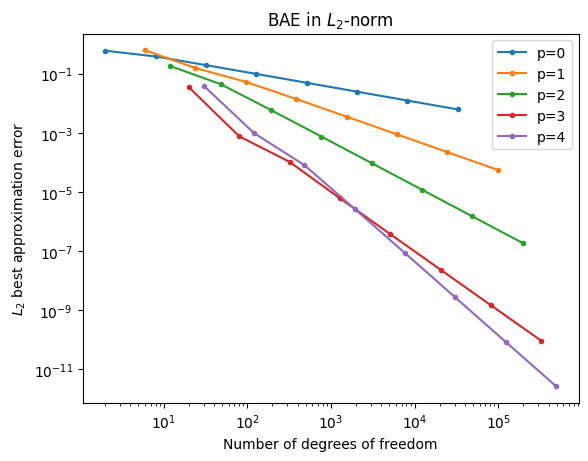
We see from these results that for the smooth u under consideration, the accuracy of its best approximation, measured per degree of freedom increases (quite dramatically) when using higher \(p\).
3.8. Stronger norms#
So far we have studied the convergence rate in the \(L_2\)-norm of the error in the projection \(Q_{hp} u\). What if we want to study the convergence in a stronger norm, such as a norm in which one measures not only how \(u - Q_{hp} u\) goes to zero in the \(L_2\)-norm, but also how its piecewise derivatives \(\partial_i( u - Q_{hp} u)\) go to zero? A standard norm that measures both the function and its first derivatives is the piecewise \(H^1\)-norm, also often called the broken \(H^1\)-norm, defined on a mesh \(\oh\) of \(\om\) by
or equivalently, in terms of \(\nabla\), the gradient operator, \( \| v \|_{H^1(\oh)}^2 = \| v \|^2_{L_2(\om)} + \sum_{K\in \oh} \| \nabla v \|^2_{L_2(\oh)}. \) Obviously, since \(\| v\|_{L_2(\om)} \le \| v \|_{H^1(\oh)}\), if the error converges at some rate in the \(H^1\)-norm, then it must converge at least at that rate in the \(L_2\)-norm. But the \(H^1\)-rate could be lower. Let us compute it.
In ngsolve, the piecewise gradient of a grid function v can be computed using the grad(v). Coefficient functions of ngsolve can also be automatically differentiated (see tutorial) using the Diff method. Hence we have all the facilities needed to compute the \(H^1\)-norm of the projection \(u - Q_{hp} u\). They are used in the function below to compute the \(H^1\)-errors on a sequence of uniformly refined meshes.
from ngsolve import grad, InnerProduct, CF

def H1ErrorsProjectOnSuccessiveRefinements(u, p=4, hcoarse=1, nrefinements=8):
    """Compute H1 errors on  on a sequence of uniformly refined meshes."""

    h1errors = []
    mesh = ng.Mesh(unit_square.GenerateMesh(maxh=hcoarse))
    gradu = CF((u.Diff(x), u.Diff(y)))

    for ref in range(nrefinements):
        W = ng.L2(mesh, order=p)
        Qu = ProjectL2(u, W)
        sqrerr = InnerProduct(grad(Qu) - gradu, grad(Qu) - gradu)
        h1errors.append(sqrt(Integrate(sqrerr, mesh)))
        mesh.ngmesh.Refine()

    return np.array(h1errors)

h1errs = H1ErrorsProjectOnSuccessiveRefinements(u, p=4)
TabulateRate('H1norm(Qu-u)', h1errs)
+-------+----------------+------+
|   h   |  H1norm(Qu-u)  | rate |
+-------+----------------+------+
|   1   | 0.886203399472 |  *   |
|  1/2  | 0.047171985649 | 4.23 |
|  1/4  | 0.006777775135 | 2.80 |
|  1/8  | 0.000445745199 | 3.93 |
|  1/16 | 0.000028167079 | 3.98 |
|  1/32 | 0.000001765061 | 4.00 |
|  1/64 | 0.000000110388 | 4.00 |
| 1/128 | 0.000000006900 | 4.00 |
+-------+----------------+------+
We observe that the convergence rate in the stronger norm is slower. By experimenting with more degrees, one observes that the rate of convergence in the \(H^1\)-norm is approximately \(p\) (which is one order less than the rate of \(p+1\) that we have seen for the \(L_2\)-norm).
3.9. Summary#
We have seen
trial and test functions in variational equations,
orthogonal projections and distance minimizers,
assembly of stiffness matrix of a bilinear form,
sparse matrix inversion facility,
how to integrate expressions over a mesh,
how to perform uniform refinement of an unstructured mesh,
how to compute and tabulate convergence rates,
how best approximation errors decrease with \(h\) and \(p\), and
that convergence rates are lower in stronger norms.