1.4. Vector guided modes of a step-index fiber#
The LP modes computed in Notebook 1.1 and Notebook 1.2 are solutions to the scalar Helmholtz equation. This is the weakly guiding approximation, which assumes the refractive index contrast between core and cladding is small (\(n_\text{core} \approx n_\text{clad}\)). Under this approximation, the two polarization components of the electromagnetic field decouple, and each satisfies an independent scalar equation.
For fibers with stronger index contrast, or whenever higher accuracy is required, the full vector structure of light must be retained. The true fiber modes are solutions of Maxwell’s equations, not the scalar Helmholtz equation, and are called vector modes. This notebook shows how to compute them, both semi-analytically and numerically. The implemented numerical method is taken from [1].
The vector waveguide eigenproblem#
We take the fiber’s axis to be \(z\) and its transverse cross-section to lie in the \((x, y)\)-plane. The time-harmonic Maxwell equations in a nonmagnetic medium with refractive index \(n\) are
A time-harmonic mode propagating along \(z\) takes the ansatz form
where \(\beta\) is the propagation constant and \(E\) is to be determined. In other words, the real time-dependent electric field is the real part of \(E(x, y) e^{i (\beta z - \omega t)}\). This is the waveguide mode ansatz we use throughout this codebase (but note that the other sign convention with \(e^{i (-\beta z + \omega t)}\) is also often used in the literature).
The vector field \(E\) splits into a transverse part \(E_\tau\) (a 2D vector field in the \(xy\)-plane) and a longitudinal component \(E_z\). Introducing the scaled longitudinal variable \(\varphi = i\beta E_z\), and using a characteristic length \(L\) for the cross-section (equal to \(r_\text{core}\) for a step-index fiber, but potentially different for microstructured fibers in later notebooks), substituting the ansatz (2) into the Maxwell system (1), eliminating \(\hat H\), and nondimensionalizing as in the scalar case (see Notebook 1.2) yields the coupled system
where:
\(Z^2 = L^2(k^2 n_0^2 - \beta^2)\) is the nondimensional eigenvalue and \(n_0 = n_\text{clad}\) is the cladding refractive index, which is assumed to be the index of the surrounding medium extending to infinity.
\(\mathcal{V}(x,y) = L^2 k^2\bigl(n_0^2 - n(x,y)^2\bigr)\) is the index well. It is zero in the infinite cladding and negative inside the core where \(n > n_0\).
The 2D differential operators are
\(\operatorname{curl}(F_\tau) = \partial_x F_y - \partial_y F_x\) (scalar-valued), and
\(\operatorname{rot}\phi = R\,\operatorname{grad}\phi\) where \(R\) is the 90^\circ rotation \(R(F_x, F_y) = (F_y, -F_x)\).
This is a mixed eigenproblem for the eigenvalue \(Z^2\). For guided modes, \(\beta > kn_0\), so \(Z^2 < 0\). The guided modes therefore lie at \(Z^2 \in (-V^2, 0)\), where \(V = Lk\sqrt{n_\text{core}^2 - n_\text{clad}^2}\) is the fiber \(V\)-number — the same range as in the scalar case of Notebook 1.2.
Note that in the weakly guiding limit (\(n_\text{core} \approx n_\text{clad}\), so \(\mathcal{V} \approx 0\) inside the core), the constraint equation forces \(\varphi \approx 0\) and the first equation reduces to the scalar Helmholtz equation for each component of \(E_\tau\) separately, recovering the LP modes.
Mode classification#
For a radially symmetric fiber, vector modes are classified by an azimuthal order \(m \ge 0\):
\(m = 0\): The electric and magnetic fields are azimuthally symmetric. These split into two families:
TE\(_{0n}\) (transverse electric): the electric field lies purely in the azimuthal direction (\(E_z = 0\), so \(\varphi = 0\)).
TM\(_{0n}\) (transverse magnetic): the magnetic field lies purely in the azimuthal direction (\(H_z = 0\)).
\(m \ge 1\): Hybrid modes, denoted HE\(_{mn}\) and EH\(_{mn}\), in which both \(E_z\) and \(H_z\) (equivalently, both \(E_\tau\) and \(\varphi\)) are nonzero. Each hybrid mode comes in a degenerate pair related by a \(90^\circ\) rotation in the cross-section.
In the weakly guiding limit, mode groups become nearly degenerate and combine into the LP modes of Notebook 1.1:
The splitting of these groups is precisely the correction that the scalar LP approximation misses.
Characteristic equations#
As with LP modes, the exact propagation constants of vector modes can be found analytically by solving characteristic equations in terms of Bessel functions. Using \(U = r_\text{core}\sqrt{k^2 n_\text{core}^2 - \beta^2}\) (the same \(X\) as in Notebook 1.1) and \(W = r_\text{core}\sqrt{\beta^2 - k^2 n_\text{clad}^2}\), with \(U^2 + W^2 = V^2\), the equations are:
TE modes (\(m=0\)):
TM modes (\(m=0\)):
Hybrid modes (\(m \ge 1\)):
The nondimensional eigenvalue from [1] relates to \(W\) by \(Z^2 = -W^2\) for guided modes (where \(W\) is real), consistent with \(Z\) being purely imaginary on the imaginary axis as in Notebook 1.2. Standard references for these equations include [2], [3]. Note that unlike the LP characteristic equation (which depends on \(n\) only through \(V\)), the TM and hybrid equations depend explicitly on both \(n_\text{core}\) and \(n_\text{clad}\) separately.
Semi-analytical computation#
The StepIndexExact class provides vec_propagation_constants(m) to find all guided vector mode roots for a given azimuthal order \(m\). The method returns \(Y\)-values (where \(Y = W = r_\text{core}\sqrt{\beta^2 - k^2 n_\text{clad}^2}\)), which are real and positive for guided modes and related to the eigenvalue in [1] by \(Z^2 = -Y^2\).
import warnings
warnings.filterwarnings('ignore', category=RuntimeWarning)
warnings.filterwarnings('ignore', category=UserWarning)
from fibermode import StepIndexExact

f = StepIndexExact('Nufern_Yb')
print(f)
STEP INDEX FIBER ATTRIBUTES: -------------------------------------------
ks:                  5.90525e+06                       signal wavenumber
wavelength:            1.064e-06                       signal wavelength
V:                       4.42894                       V-number of fiber
ncore:                   1.45097                   core refractive index
nclad:                   1.44973               cladding refractive index
NA:                         0.06                      numerical aperture
rcore:                  1.25e-05                             core radius
rclad:                    0.0002                         cladding radius
------------------------------------------------------------------------
TE and TM modes (\(m = 0\))#
For \(m = 0\), the TE and TM families are computed separately by passing m0name.
Y0TE = f.vec_propagation_constants(0, m0name='TE')
Y0TM = f.vec_propagation_constants(0, m0name='TM')
Y0TE
[([3.1917501724134585],
  np.float64(3.1916126395860496),
  np.float64(3.191982594544141))]
print('TE modes:')
for yab in Y0TE:
    for y in yab[0]:
        print('  Y = %18.12f   Z² = %18.12f   beta = %22.12f'
              % (y, -y**2, f.ZtoBeta(1j * y).real))

print('TM modes:')
for yab in Y0TM:
    for y in yab[0]:
        print('  Y = %18.12f   Z² = %18.12f   beta = %22.12f'
              % (y, -y**2, f.ZtoBeta(1j * y).real))
TE modes:
  Y =     3.191750172413   Z² =   -10.187269163101   beta =   8564823.696138797328
TM modes:
  Y =     3.191201078384   Z² =   -10.183764322682   beta =   8564822.386655895039
Hybrid modes (\(m \ge 1\))#
For each \(m \ge 1\), the roots of the hybrid characteristic equation give both HE and EH modes. Each root corresponds to a degenerate pair of modes (the two orientations of the hybrid mode).
Ys = [Y0TE + Y0TM]  # m=0

for m in range(1, 6):
    Ys.append(f.vec_propagation_constants(m))
print('GUIDED VECTOR MODES' + ' ='*30)
print('          Y-values        Z² values              beta-values')
print('-' * 70)

print('  m = 0  TE')
for yab in Y0TE:
    for y in yab[0]:
        print('  %20.12f %20.12f  %24.12f' % (y, -y**2, f.ZtoBeta(1j*y).real))

print('  m = 0  TM')
for yab in Y0TM:
    for y in yab[0]:
        print('  %20.12f %20.12f  %24.12f' % (y, -y**2, f.ZtoBeta(1j*y).real))

for m in range(1, 6):
    if Ys[m]:
        print('  m = %d  HYBRID (degenerate pairs)' % m)
        for yab in Ys[m]:
            for y in yab[0]:
                print('  %20.12f %20.12f  %24.12f' % (y, -y**2, f.ZtoBeta(1j*y).real))

print('=' * 70)
GUIDED VECTOR MODES = = = = = = = = = = = = = = = = = = = = = = = = = = = = = =
          Y-values        Z² values              beta-values
----------------------------------------------------------------------
  m = 0  TE
        3.191750172413     -10.187269163101      8564823.696138797328
  m = 0  TM
        3.191201078384     -10.183764322682      8564822.386655895039
  m = 1  HYBRID (degenerate pairs)
        1.287547323034      -1.657778109053      8561636.304071478546
        1.805596864133      -3.260180035768      8562235.197395928204
        3.977130884564     -15.817570072951      8566927.037845231593
  m = 2  HYBRID (degenerate pairs)
        3.191278323488     -10.184257337967      8564822.570856899023
======================================================================
Comparing with the LP propagation constants from Notebook 1.1, the LP\(_{11}\) group (three nearly equal \(\beta\) values) splits into the TE\(_{01}\), TM\(_{01}\), and HE\(_{21}\) modes, with a small but nonzero separation. This splitting is proportional to \((n_\text{core}/n_\text{clad})^2 - 1\) and vanishes in the weakly guiding limit.
Visualizing mode profiles#
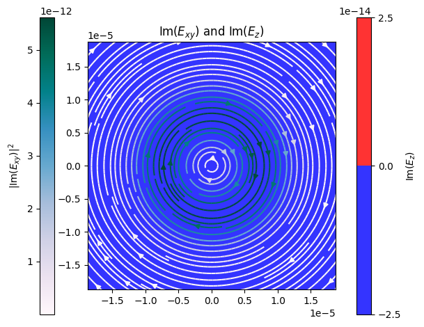
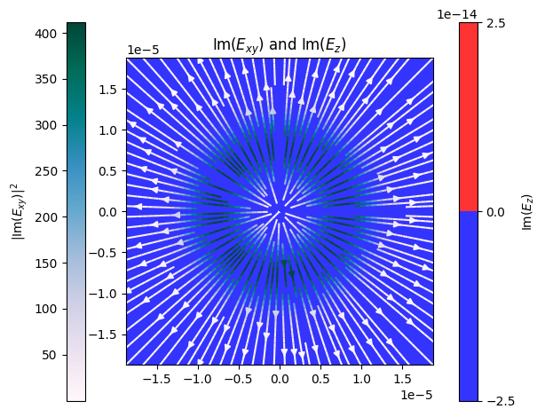
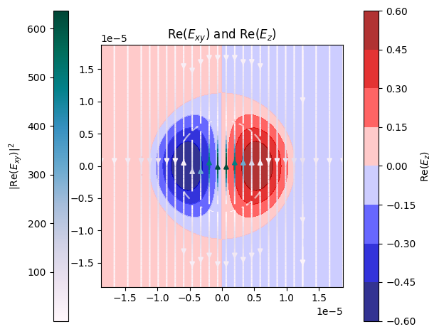
The transverse electric field \(E_\tau\) for each guided vector mode is visualized using visualize_vec_Emode.
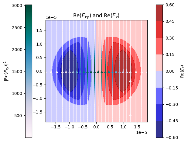
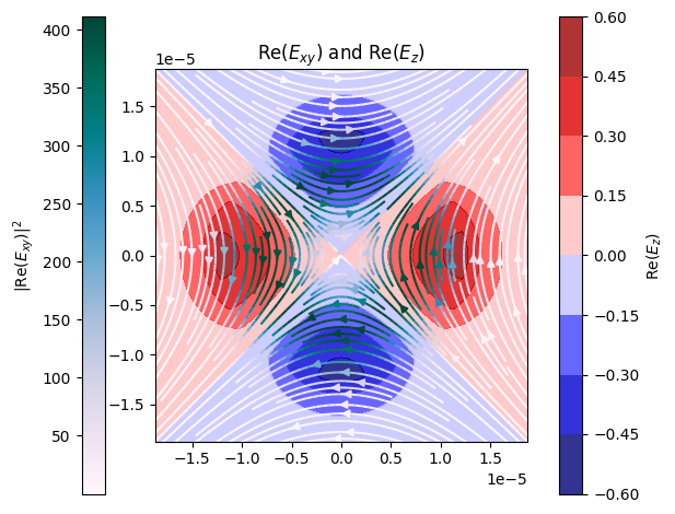
Reading the plots. Each plot shows a 2D color map of the real part of one or both components of \(E_\tau\) over the fiber cross-section. The spatial axes \((x, y)\) are the nondimensional transverse coordinates scaled by the core radius \(L = r_\text{core}\), so the core-cladding interface lies at the unit circle \(x^2 + y^2 = 1\). The color bar on the right gives the field amplitude in arbitrary (normalized) units: the color scale is centered at zero (white), with positive values in one color and negative values in the opposite color. For hybrid modes called with real=True, the displayed field is the real part of a particular phase of the complex-valued mode; the imaginary part (the second polarization orientation) is the same pattern rotated by \(90^\circ\).
TE modes (\(m=0\), \(\varphi=0\))#
for yab in Y0TE:
    for y in yab[0]:
        print('TE  Y = %.8f   beta = %.8f' % (y, f.ZtoBeta(1j*y).real))
        f.visualize_vec_Emode(0, y, m0name='TE')
TE Y = 3.19175017 beta = 8564823.69613880
TM modes (\(m=0\))#
for yab in Y0TM:
    for y in yab[0]:
        print('TM  Y = %.8f   beta = %.8f' % (y, f.ZtoBeta(1j*y).real))
        f.visualize_vec_Emode(0, y, m0name='TM')
TM Y = 3.19120108 beta = 8564822.38665590
Hybrid modes (\(m \ge 1\))#
For each azimuthal order \(m\), modes are shown in order of decreasing \(\beta\) (i.e., increasing \(Y\)). Each root of the hybrid characteristic equation represents a degenerate pair; visualize_vec_Emode shows one orientation of the pair (real=True).
for m in range(1, 6):
    for yab in Ys[m]:
        for y in yab[0]:
            print('Hybrid m=%d  Y = %.8f   beta = %.8f' % (m, y, f.ZtoBeta(1j*y).real))
            f.visualize_vec_Emode(m, y, real=True)
Hybrid m=1 Y = 1.28754732 beta = 8561636.30407148
Hybrid m=1 Y = 1.80559686 beta = 8562235.19739593
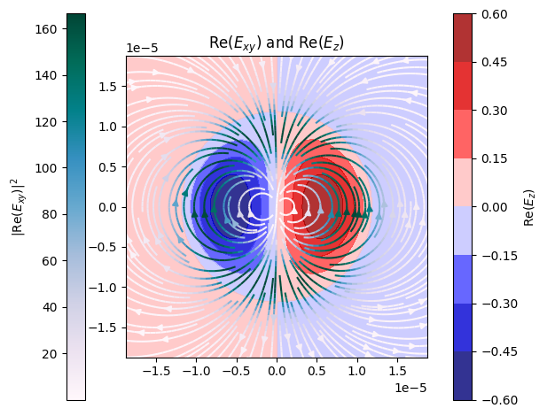
Hybrid m=1 Y = 3.97713088 beta = 8566927.03784523
Hybrid m=2 Y = 3.19127832 beta = 8564822.57085690
Numerical computation#
The semi-analytical approach above is exact but limited to radially symmetric step-index fibers. For guided modes of a general fiber geometry, we must solve the eigenproblem numerically. Here, we illustrate the use of this general facility by applying it to the step-index fiber.
The weak form of the eigenproblem [1] reads: find \(E_\tau \in \mathring{H}(\operatorname{curl}, \Omega)\) and \(\varphi \in \mathring{H}^1(\Omega)\) satisfying
for all \(F \in \mathring{H}(\operatorname{curl}, \Omega)\) and \(\psi \in \mathring{H}^1(\Omega)\). The discrete version uses Nédélec (edge) elements \(N_h\) of order \(p\) for \(E_\tau\) — which correctly enforce tangential continuity at dielectric interfaces — paired with Lagrange elements \(V_h\) of order \(p+1\) for \(\varphi\). The eigenvalues \(Z_h^2\) are found using the FEAST contour integrator.
The FEAST contour is placed in the \(Z^2\)-plane exactly as in the scalar case of Notebook 1.2. For the Nufern_Yb fiber, guided modes have \(Z^2 \in (-V^2, 0) \approx (-21, 0)\), so ctr=-10 places the search circle near the middle of this interval.
from fibermode import StepIndex
from ngsolve.webgui import Draw

fiber = StepIndex(fibername='Nufern_Yb')

# Search for guided vector modes in Z^2 in (ctr-rad, ctr+rad) = (-11, -9)
betas, zsqrs, E_tau, phi, _ = fiber.guidedvecmodes(ctr=-10, rad=1,
                                                    p=4,
                                                    niterations=100,
                                                    nrestarts=0,
                                                    stop_tol=1e-9)
ModeSolver: Checking if mesh has required regions
Mesh has  414  elements,  224  points,  and  637  edges.
Using FEAST to search for vector guided modes in
circle of radius 1 centered at -10
assuming not more than 20 modes in this interval.
System size: 11465 x 11465  Inverse type: umfpack

SpectralProj: Setting shifted trapezoidal rule quadrature on circular contour
SpectralProj: Radius=1, Center=-10+0j
SpectralProjNGR:   Making resolvent at z =  -9.076 +0.383j
SpectralProjNGR:   Making resolvent at z =  -9.617 +0.924j
SpectralProjNGR:   Making resolvent at z = -10.383 +0.924j
SpectralProjNGR:   Making resolvent at z = -10.924 +0.383j
SpectralProjNGR:   Making resolvent at z = -10.924 -0.383j
SpectralProjNGR:   Making resolvent at z = -10.383 -0.924j
SpectralProjNGR:   Making resolvent at z =  -9.617 -0.924j
SpectralProjNGR:   Making resolvent at z =  -9.076 -0.383j
=========== Starting FEAST iterations ===========
Trying with 20 vectors:

 ITERATION 1 with 20 vectors and 20 left vectors
   During kernel cleaning singular values of B-Gram:
   [1.652e+02 2.616e+00 1.578e+00 1.358e+00 9.023e-13 7.500e-13 8.631e-14
 6.742e-14 4.566e-14 2.879e-14 2.235e-14 1.439e-14 1.120e-14 9.493e-15
 7.732e-15 5.956e-15 4.332e-15 3.594e-15 2.083e-15 9.959e-16]
   Removing ew#[4, 5, 6, 7, 8, 9, 10, 11, 12, 13, 14, 15, 16, 17, 18, 19]
   Real part of computed eigenvalues:
   [-10.18730374 -10.18429193 -10.18429193 -10.18379893]
   Relative Hausdorff distance from prior iterate: 1.000e+99

 ITERATION 2 with 4 vectors and 4 left vectors
   During kernel cleaning singular values of B-Gram:
   [0.526 0.043 0.018 0.006]
   Real part of computed eigenvalues:
   [-10.18730374 -10.18429193 -10.18429193 -10.18379893]
   Relative Hausdorff distance from prior iterate: 2.112e-12


***FEAST converged with:
	Relative Hausdorff distance = 2.112e-12

============= FEAST iterations done =============
print('Computed Z² values:')
print(zsqrs)
print('\nComputed propagation constants \u03b2:')
print(betas)
Computed Z² values:
[-10.18730374-1.15416909e-13j -10.18379893+5.15620699e-14j
 -10.18429193+2.63874599e-13j -10.18429193+8.35943570e-13j]

Computed propagation constants β:
[8564823.70905581+4.31222078e-11j 8564822.39958657-1.92646871e-11j
 8564822.58378053-9.85891660e-11j 8564822.583783  -3.12326309e-10j]
The guidedvecmodes call returns all modes found in the window \(Z^2 \in (\text{ctr}-\text{rad},\, \text{ctr}+\text{rad})\) in one FEAST run. Each mode is a pair \((E_\tau, \varphi)\) of NGSolve grid functions — \(E_\tau\) living in the Nédélec space \(N_h\) and \(\varphi\) in the Lagrange space \(V_h\). Both can be visualized directly:
from ngsolve.webgui import Draw

for i in range(E_tau.m):
    print('The ', i, 'th computed mode:')
    Draw(E_tau.gridfun(i=i), vectors={'grid_size': 30});
    Draw(phi.gridfun(i=i));
The  0 th computed mode:
Warning in Webgui.Draw: function has more than 3 components, drawing Norm(cf) instead
The  1 th computed mode:
Warning in Webgui.Draw: function has more than 3 components, drawing Norm(cf) instead
The  2 th computed mode:
Warning in Webgui.Draw: function has more than 3 components, drawing Norm(cf) instead
The  3 th computed mode:
Warning in Webgui.Draw: function has more than 3 components, drawing Norm(cf) instead
Comparing numerical and exact propagation constants#
The guidedvecmodes call above searched only the window \(Z^2 \in (\text{ctr}-\text{rad},\,\text{ctr}+\text{rad}) = (-11, -9)\), so it returns only the subset of guided modes whose \(Z^2\) fall in that window. The semi-analytical computation found all guided modes across \(Z^2 \in (-V^2, 0)\).
Each hybrid mode has a degenerate pair of numerical eigenvalues converging to one exact \(\beta\). For such pairs we report the Hausdorff distance between the set of numerical values and the exact value — that is, the worst-case error across the pair. Non-degenerate modes (TE, TM) reduce to the ordinary absolute error. Both \(\beta\) and \(Z^2\) errors are shown.
import numpy as np
from collections import defaultdict

# Sort numerical modes by beta (descending), keeping beta and Z² paired
sort_idx    = np.argsort(betas.real)[::-1]
num_betas_s = betas.real[sort_idx]
num_zsqrs_s = zsqrs.real[sort_idx]

# Collect all exact modes: (beta, label, Z²)
exact = []
for yab in Y0TE:
    for y in yab[0]:
        exact.append((f.ZtoBeta(1j * y).real, 'TE',        float(-y**2)))
for yab in Y0TM:
    for y in yab[0]:
        exact.append((f.ZtoBeta(1j * y).real, 'TM',        float(-y**2)))
for m in range(1, 6):
    for yab in Ys[m]:
        for y in yab[0]:
            b = f.ZtoBeta(1j * y).real
            exact.append((b, f'hybrid m={m}', float(-y**2)))  # degenerate pair: two entries
            exact.append((b, f'hybrid m={m}', float(-y**2)))

exact.sort(key=lambda x: -x[0])
exact_betas_arr = np.array([e[0] for e in exact])

# Match each numerical beta to nearest exact, group by exact index
groups_beta = defaultdict(list)
groups_zsq  = defaultdict(list)
for b_num, z2_num in zip(num_betas_s, num_zsqrs_s):
    idx = np.argmin(np.abs(exact_betas_arr - b_num))
    groups_beta[idx].append(b_num)
    groups_zsq[idx].append(z2_num)

in_window  = sum(1 for _, _, z2 in exact if -11 < z2 < -9) // 1
out_window = len(exact) - in_window
print(f'Search window: Z² ∈ (-11, -9)')
print(f'Exact modes in window: {in_window},  outside window (not sought): {out_window}')
Search window: Z² ∈ (-11, -9)
Exact modes in window: 4,  outside window (not sought): 6
from scipy.spatial.distance import directed_hausdorff

def hausdorff(nums, exact_val):
    """Hausdorff distance between a set of points and a single exact value."""
    u = np.array(nums).reshape(-1, 1)
    v = np.array([[exact_val]])
    return max(directed_hausdorff(u, v)[0], directed_hausdorff(v, u)[0])

hdr = f'{"Mode":<20}  {"mult":>4}  {"β_exact":>22}  {"dH_rel(β)":>12}  {"Z²_exact":>12}  {"dH(Z²)":>12}'
print(hdr)
print('-' * len(hdr))

for idx in sorted(groups_beta.keys(), key=lambda i: -exact[i][0]):
    b_ex    = exact[idx][0]
    label   = exact[idx][1]
    z2_ex   = exact[idx][2]

    dH_beta = hausdorff(groups_beta[idx], b_ex) / abs(b_ex)
    dH_z2   = hausdorff(groups_zsq[idx],  z2_ex)
    mult    = len(groups_beta[idx])

    print(f'{label:<20}  {mult:>4}  {b_ex:>22.12f}  {dH_beta:>12.2e}  {z2_ex:>12.6f}  {dH_z2:>12.2e}')
Mode                  mult                 β_exact     dH_rel(β)      Z²_exact        dH(Z²)
--------------------------------------------------------------------------------------------
TE                       1    8564823.696138797328      1.51e-09    -10.187269      3.46e-05
hybrid m=2               2    8564822.570856899023      1.51e-09    -10.184257      3.46e-05
TM                       1    8564822.386655895039      1.51e-09    -10.183764      3.46e-05
References#
[1] J. Gopalakrishnan, J. Grosek, G. Pinochet-Soto, and P. Vandenberge, “Adaptive resolution of fine scales in modes of microstructured optical fibers,” SIAM Journal on Scientific Computing, 2025. Open Access, DOI: 10.1137/24M1651605
[2] A. W. Snyder and J. D. Love, Optical Waveguide Theory, Chapman and Hall, London, 1983.
[3] D. Marcuse, Theory of Dielectric Optical Waveguides, 2nd ed., Academic Press, 1991.