1.3. Leaky modes of a step-index fiber#
Step-index fibers typically have guided modes and leaky modes. Leaky modes are also called resonances or quasinormal modes. They are defined as a nontrivial function \(\varphi\) that satisfies, together with some complex number \(\beta\), the following Helmholtz equation on the entire plane containing a fiber’s transverse cross section,
Instead of a boundary condition near the fiber boundary, leaky modes \(\varphi\) satisfy the condition that they are outgoing at infinity.
The definition of an outgoing solution of \(\Delta \varphi + (k^2 n^2 -\beta^2) \varphi = 0\) when \(\kappa^2 = k^2 n^2 -\beta^2\) is real is simple and can be found in textbooks. One equivalent characterization of outgoing \(\varphi\) when \(\kappa\) is real is that \(\varphi\) satisfies the Sommerfeld radiation condition. For complex \(\kappa\) however, the definition of outgoing is more delicate. A mathematically correct approach is to use complex analysis to define an outgoing \(\varphi\) as a meromorphic continuation of an outgoing solution obtained in the real \(\kappa\) case. Leaky modes have complex \(\beta\). In our numerical methods to compute leaky modes, the perfectly matched layer (PML) selects outgoing solutions by damping them exponentially. In our semi-analytical methods, we select Hankel functions that are outgoing to match the fiber core solutions.
The modal solutions of (1) yield Helmholtz solutions \(u(x, y,z) = \varphi(x, y) e^{i \beta z}\) propagating along the longitudinal (\(z\)) direction of the fiber. Confinement loss (CL), usually expressed in decibels (dB) per meter, is defined as
where \(P(z)\) is the power in the fiber cross section at \(z\). For a leaky mode, viewing the power as proportional to \(|e^{i\beta z}|^2\), its CL can be estimated from the imaginary part of the propagation constant \(\text{Im}(\beta)\) by
For this reason, computing the imaginary part of \(\beta\) for leaky modes is important for correctly estimating confinement losses.
In this notebook we present semi-analytical facilities based on exact leaky mode expressions available for step-index fibers, as well as fully numerical facilities using finite elements to compute the same modes approximately.
Semi-analytical leaky mode finder#
Leaky modes are computed in the non-dimensional \(Z\)-plane, while the guided modes are computed in the non-dimensional \(X\)-plane. Recall from Notebook 1.1 that non-dimensional \(X\)-values are related to dimensional \(\beta\)-values by \(X = r_{\text{core}}\sqrt{n_{\text{core}}^2 k^2-\beta^2}.\) The new non-dimensional variable \(Z\) is related to \(X\) via the fiber V-number:
The facility to compute \(Z\) values for leaky modes, which then give the leaky \(\beta\) values, is shown next:
from fibermode import StepIndexExact
import numpy as np
import logging,  warnings
warnings.filterwarnings('ignore', category=RuntimeWarning)
warnings.filterwarnings('ignore', category=UserWarning)
f = StepIndexExact('Nufern_Yb')
z = f.leaky_propagation_constants(0)
Z = np.array(z)
Z
array([ 5.35183517-1.33494282j,  9.06190986-1.63804197j,
       12.47195866-1.87353665j])
Using equation (2), we can compute \(\beta\) values from these \(Z\) values. The StepIndexExact class has a method to do just that. Here are the corresponding dimensional \(\beta\) values:
f.ZtoBeta(Z) # convert to dimensional propagation constants
array([8550972.49352094 +5347.24223594j, 8531280.45716445+11135.52043093j,
       8504014.47232996+17585.42381389j])
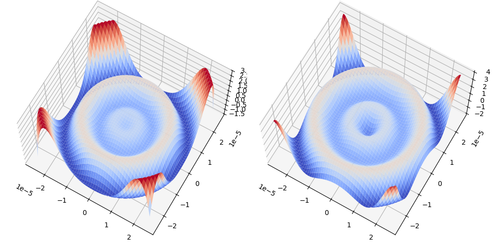
For each value of \(Z\) (or \(\beta\)), the accompanying mode function can be visualized as shown next.
X, Y, F, mode, = f.visualize_leaky_mode(z[0], 0)
import matplotlib.pyplot as plt
from matplotlib import cm

fig, ax = plt.subplots(1, 2, subplot_kw={'projection': '3d'})
fig.set_size_inches(10, 7)
fig.tight_layout()

ax[0].plot_surface(X, Y, F.real, cmap=cm.coolwarm, linewidth=0);
ax[0].view_init(azim=-60, elev=68)

ax[1].plot_surface(X, Y, F.imag, cmap=cm.coolwarm);
ax[1].view_init(azim=-60, elev=68)
Numerical leaky mode finder#
Using finite elements and the perfectly matched layer (PML), the StepIndex class of fibermode provides numerical routines to compute the same leaky modes. PML allows us to truncate the infinite domain \(\mathbb R^2\) to a bounded circular computational domain. It is important to note that the numerical modes are only accurate in the region without PML since PML deforms and attenuates the mode within it to eliminate potential reflections from the artificial boundary.
from fibermode import StepIndex
from ngsolve.webgui import Draw
Using the same class StepIndex that we used for numerical guided mode computation in Notebook 1.2, we can now compute leaky modes by specifying PML parameters.
fiber = StepIndex(fibername='Nufern_Yb',
                  R=2,
                  Rout=8,   # PML is set in R < r < Rout
                  refine=1)
ModeSolver: Checking if mesh has required regions
Mesh has  1184  elements,  609  points,  and  1792  edges.
Next, we call the leakymode method, an algorithm applicable to many fibers. It uses a frequency-dependent perfectly matched layer (PML) and a polynomial eigensolver described in [1], which builds on the frequency-dependent PML approach of [2]. The PML strength and an approximate search region for finding leaky modes in the \(Z\)-plane must be given as inputs.
zh, y, yl, beta, _, _ = fiber.leakymode(p=3,          # degree of finite  elements
                                        rad=0.3,      # search radius in Z-plane
                                        ctr=5.4-1.3j, # center of search circle in Z-plane
                                        alpha=5,      # PML strength parameter
                                        verbose=False)
ModeSolver.leakymode called on object with these settings:

StepIndex (ModeSolver) Object:------------------------------------------
Nondimensional Computational Parameters:
  Geometry consists of circular core (radius = 1), an annular
  cladding layer 1<r<R=2, and an outer layer R<r<Rout=8.
  Max mesh sizes: 0.3 (core), 3 (cladding), 3 (outer)
  Mesh curved by order 3
Physical Parameters:
  Wavelength = 1.064e-06 meters
  Refractive indices: 1.44973 (cladding), 1.45097 (core)
  No curvature set
  No temperature set
Included fiber object:
STEP INDEX FIBER ATTRIBUTES: -------------------------------------------
ks:                  5.90525e+06                       signal wavenumber
wavelength:            1.064e-06                       signal wavelength
V:                       4.42894                       V-number of fiber
ncore:                   1.45097                   core refractive index
nclad:                   1.44973               cladding refractive index
NA:                         0.06                      numerical aperture
rcore:                  1.25e-05                             core radius
rclad:                    0.0002                         cladding radius
------------------------------------------------------------------------
Set freq-dependent PML with p= 3  alpha= 5 and thickness=6.000
   Normalizing by M-norms: max=3.4e-03, min=3.4e-03
   Normalizing by M-norms: max=1.3e+03, min=1.3e+03
Results:
 Z: [5.34915796-1.32839913j]
 beta: [8550976.67463514+5318.36642726j]
 CL dB/m: [46194.74384197]
Mode boundary L² norm = 1.0e-10
We see that the computed \(Z\)-value is close to one of the values found in the previous section through semi-analytical computation. The accompanying numerical leaky modes can be visualized using ngsolve as follows.
yh = y.gridfun()
yh_real = -10 * yh.real
Draw(yh_real, fiber.mesh, deformation=True, euler_angles=[-55, 10,10]);
This plot shows that in the non-PML region \(r < R\), the numerically found mode indeed approximates the semi-analytical mode computed earlier by different methods. (In the PML region \(R < r < R_{\text{out}}\), the mode decays rapidly.)
Spectral locations in the complex plane#
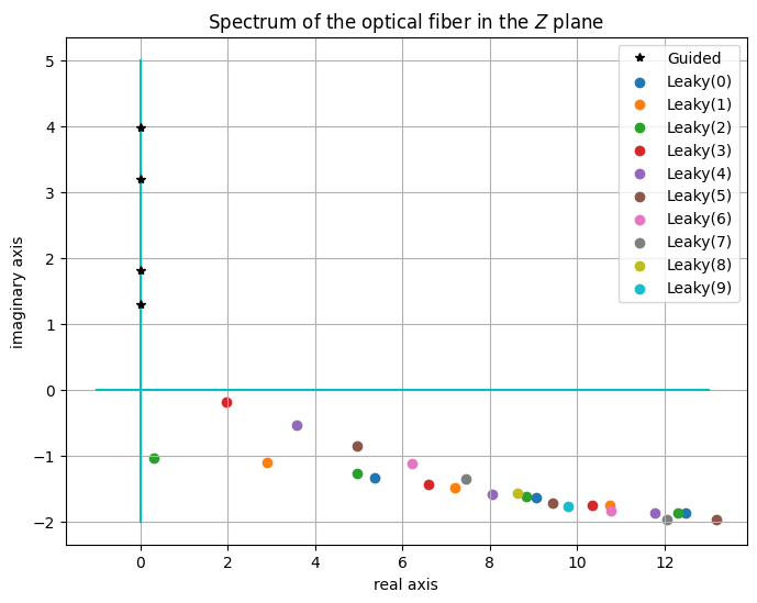
For the fiber we’ve been considering, let us examine what the computations show us about the structure of the spectrum in the complex plane. We can visualize the spectrum either in the \(\beta\)-plane or in the non-dimensional \(Z\)-plane. We begin with the \(Z\)-plane. We will be able to discern the spectral structure when we plot all the computed \(Z\) values together.
# compute many leaky modes

Z = [np.array(z)]
for i in range(1, 11):
  Z += [np.array(f.leaky_propagation_constants(i))]
print('Leaky mode Z values:')
[print('l=%2d:'%i, z) for i, z in enumerate(Z)];
Leaky mode Z values:
l= 0: [ 5.35183517-1.33494282j  9.06190986-1.63804197j 12.47195866-1.87353665j]
l= 1: [10.73969427-1.76141964j  7.20192238-1.49241378j  2.90332447-1.10196391j]
l= 2: [ 4.94983851-1.27807156j  8.83440294-1.62883323j 12.30887507-1.87197156j
  0.30443515-1.03769972j]
l= 3: [10.34886626-1.75223106j  6.58684234-1.43790073j  1.95779333-0.1854324j ]
l= 4: [ 8.06126037-1.58406974j 11.78789593-1.86605333j  3.58395439-0.54550353j]
l= 5: [ 4.95242123-0.85256877j  9.44561168-1.71940686j 13.17399551-1.97232174j]
l= 6: [ 6.22542787-1.12064721j 10.77205962-1.84594073j]
l= 7: [ 7.44661469-1.36014393j 12.05787335-1.96514566j]
l= 8: [8.63476045-1.57775829j]
l= 9: [9.7998061-1.77800664j]
l=10: [10.94769637-1.96408165j]
# compute all guided modes

X = []
for i in range(3):
    X += f.propagation_constants(i, loglevel=logging.ERROR)
Zguided2 = np.array(X)**2 - f.fiberV()**2
Zguided = 1j  * np.sqrt(-Zguided2)
Zguided
array([0.+3.97727885j, 0.+1.28813166j, 0.+3.19175017j, 0.+1.80585711j])
fig, ax = plt.subplots()
fig.set_size_inches(8, 6)
ax.set_title('Spectrum of the optical fiber in the $Z$ plane')
ax.set_xlabel('real axis')
ax.set_ylabel('imaginary axis')

# draw real and imaginary axis of the complex plane
ax.plot([0, 0], [-2, 5], 'c');
ax.plot([-1, 13], [0, 0], 'c');

# plot the guided mode eigenvalues
ax.plot(Zguided.real, Zguided.imag, 'k*', label='Guided')

# plot the leakymode eigenvalues
for l in range(10):
    lab = 'Leaky(%d)' % l
    ax.scatter(np.array(Z[l]).real, np.array(Z[l]).imag, label=lab)
ax.grid(True); ax.legend();
The physical propagation constants \(\beta\) are large and are located in a different region in the complex plane. Let us visualize the same spectrum in the \(\beta\)-plane.
betas = []
for z in Z:
    betas.append(f.ZtoBeta(np.array(z)))
print('Leaky mode beta values:')
[print('l=%2d:'%i, beta) for i, beta in enumerate(betas)];
Leaky mode beta values:
l= 0: [8550972.49352094 +5347.24223594j 8531280.45716445+11135.52043093j
 8504014.47232996+17585.42381389j]
l= 1: [8518971.9110389 +14211.74939379j 8542445.36359659 +8052.58748582j
 8558319.71526637 +2392.51359413j]
l= 2: [8552466.1504492  +4734.07147447j 8532795.79126769+10793.00667804j
 8505532.35292016+17337.88359689j 8561384.52440338  +236.15789334j]
l= 3: [8522054.21688928+13618.20382951j 8545561.16137416 +7093.25476739j
 8559596.69914123  +271.44330587j]
l= 4: [8537637.86690138 +9572.37026789j 8510244.2460348 +16542.39148956j
 8556325.54136906 +1462.35465357j]
l= 5: [8552116.63574704 +3159.75460351j 8528720.32274048+12187.22541705j
 8497384.25267688+19569.96234247j]
l= 6: [8546989.70752667 +5224.02098757j 8518826.15478818+14938.83465687j]
l= 7: [8540960.76096976 +7589.56700117j 8507968.55076558+17824.59053845j]
l= 8: [8534041.49860126+10216.82579231j]
l= 9: [8526240.56508639+13078.96125833j]
l=10: [8517564.38458725+16156.48313268j]
fig, ax = plt.subplots()
fig.set_size_inches(8, 6)
ax.set_title('Spectrum of the optical fiber in the $\\beta$ plane')
ax.set_xlabel('real part')
ax.set_ylabel('imaginary part')
ax.plot(f.XtoBeta(X), [0]*len(X), 'k*', label='Guided')
for l in range(10):
    lab = 'Leaky(%d)' % l
    ax.scatter(betas[l].real, betas[l].imag, label=lab)
ax.grid(True); ax.legend();
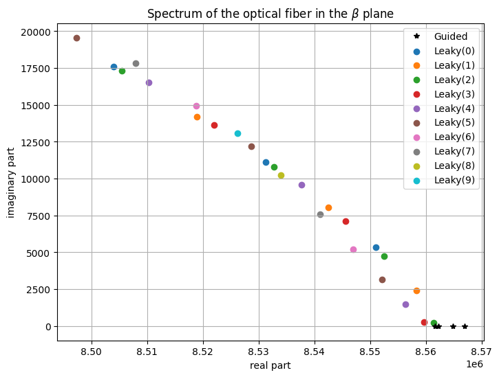
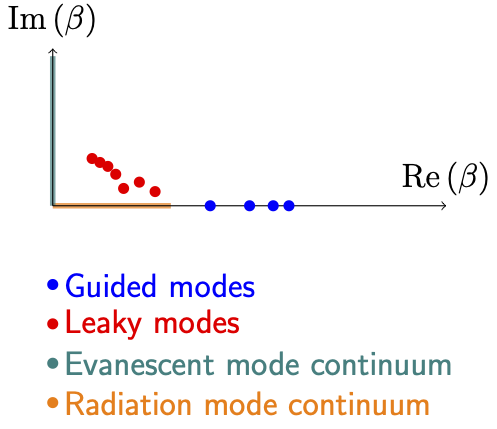
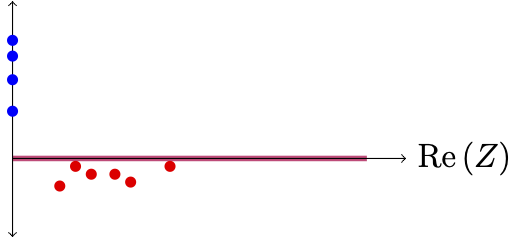
These plots show the typical structure of the spectrum of a step-index optical fiber. To reinforce this point, we conclude by showing schematic diagrams of the spectrum in both the \(\beta\)-plane and the \(Z\)-plane.
Typical diagrams of propagation constant locations (\(\beta\)-values) in the complex plane take the following form, where we have separated guided, leaky, evanescent, and radiation parts of the spectrum by different colors:
In contrast, the non-dimensional \(Z\) value locations in the complex plane have a different structure. Since the optical \(Z^2\) value can be equivalently viewed as a Schrödinger spectral point, and since the essential spectrum of the Laplacian is unperturbed by a bounded potential well, we first mark the essential spectrum in the plot (in red). The guided modes are now on the imaginary axis in the \(Z\)-plane, while the leaky modes hover just below the real axis.
References#
[1] J. Gopalakrishnan, C. Parker, and P. Vandenberge, “Computing leaky modes of optical fibers using a FEAST algorithm for polynomial eigenproblems,” Wave Motion, vol. 101, p. 102826, 2021. DOI: 10.1016/j.wavemoti.2021.102826
[2] L. Nannen and M. Wess, “Computing scattering resonances using perfectly matched layers with frequency dependent scaling functions,” BIT Numer. Math., vol. 58, pp. 373–395, 2018. DOI: 10.1007/s10543-017-0694-1