1. Elements on 1D domains

In this activity, we become familiar with a computational object that can represent members of simple finite element spaces on one-dimensional (1D) domains. The spaces are vector spaces of functions on the spatial domain. We see how distinct finite elements on a mesh are glued together to form such a space. The glued function space is often called a global finite element space to contrast it with the spaces on each individual finite element, referred to as local finite element spaces. This leads to the concept of coupling degrees of freedom and local degrees of freedom of global finite element spaces.

We start by importing the Python objects we use in this notebook.

import ngsolve as ng
from ngsolve.meshes import Make1DMesh
from ngsolve import H1, x, sin, Discontinuous, GridFunction
import matplotlib.pyplot as plt
import numpy as np
from matplotlib.colors import TABLEAU_COLORS as tc
colors = [tc[key] for key in tc]    

1.1. One element

We create a mesh of the unit interval \([0, 1]\) consisting of a single finite element on the same interval, as follows.

mesh1 = Make1DMesh(1) # one element mesh of [0, 1]
for p in mesh1.vertices:
    print(p.point)    # confirm the mesh point coordinates

(0.0,)
(1.0,)

In higher dimensions, the printed tuple p.point will show more coordinates.

The quadratic Lagrange finite element on this single element is made in the V1 object below using the ngsolve facility H1. (The name H1 refers to a Sobolev space related to the Lagrange finite elements.) The ndof attribute stores the number of degrees of freedom of the element. In this case, we get the expected number of three degrees of freedom for the quadratic Lagrange element.

V1 = H1(mesh1, order=2) # set degree using the keyword "order"
V1.ndof

3

Functions of finite element spaces are represented by GridFunction objects in ngsolve.

v = ng.GridFunction(V1)

If \(\theta_i(x)\) denote the shape functions of this finite element, then any function in the finite element space takes the form

\[ v(x) = \sum_i v_i \theta_i(x) \]

for some numbers \(v_i\). The GridFunction object v represents this function \(v\) and contains the numbers \(v_i\) in its data attribute v.vec. By printing out v.vec we thus have complete information on the function, provided we know the shape functions \(\theta_i\). Similarly, by setting the array v.vec, we can represent any function in the finite element space as we wish.

Not all finite element codes use the same shape functions (even if the space they span is a classical finite element space). Let us acquaint ourselves with the Lagrange shape functions \(\theta_i(x)\) used by ngsolve. We need a small routine to evaluate the finite element function at many points (say a hundred, as set below) within an element and plot the result.

def plot1D(w, msh, style='k', title=None):  
  """
  Utility to plot 1D finite element functions
  """
  pts = [vtx.point[0] for vtx in msh.vertices]
  ev = [e.vertices for e in msh.Elements(ng.VOL)]
  for i in range(len(ev)):
    a = pts[ev[i][0].nr] 
    b = pts[ev[i][1].nr] 
    aa = min(a, b) + 0.01 * abs(b-a)
    bb = max(a, b) - 0.01 * abs(b-a)
    xs = np.linspace(aa, bb, num=100)
    ws = [w(msh(x)) for x in xs]
    plt.plot(xs, ws, style, alpha=0.5, lw=3)
  plt.xlabel('x'); plt.title(title)

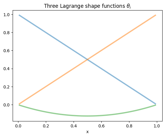
In three distinct colors, we see the three shape functions of the quadratic Lagrange element used within ngsolve. We discover that the Lagrange shape functions in ngsolve are not exactly the shape functions generated by the degrees of freedom of the principal lattice. But note that (see exercises) the same finite element can admit many distinct unisolvent degrees of freedom.

for i in range(3):
  v.vec[:] = 0
  v.vec[i] = 1
  plot1D(v, mesh1, style=colors[i], title='Three Lagrange shape functions $\\theta_i$')

1.2. How elements are glued

mesh2 = Make1DMesh(2)  # two element mesh
for p in mesh2.vertices:
    print(p.point)     # this mesh now has 3 points

(0.0,)
(0.5,)
(1.0,)

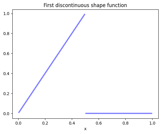
On this mesh of two elements, let us start by examining two independent quadratic Lagrange elements, where functions of one element are not glued to the next element. This is achieved using the Discontinuous facility in ngsolve. As expected we now find a space of dimension \(3 + 3 = 6\). This space is called the discontinuous Galerkin space or the DG space.

V2 = Discontinuous(H1(mesh2, order=2))
V2.ndof

6

v = GridFunction(V2)
v.vec[:] = 0; v.vec[0] = 1
plot1D(v, mesh2, style='b', title='First discontinuous shape function')

v.vec[:] = 0; v.vec[4] = 1
plot1D(v, mesh2, style='k:', title='Fourth discontinuous shape function')

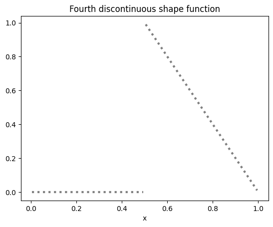
If we glue these first and fourth functions together we get a continuous function. The global Lagrange finite element space accomplishes this by coalescing the first and fourth degrees of freedom into one, thereby merging the above two shape functions into one global shape function corresponding to the fused global degree of freedom. This global Lagrange finite element space can be obtained in ngsolve by simply omitting the adjective Discontinuous from the prior space definition.

V = H1(mesh2, order=2) # omitted "Discontinuous"
V.ndof

5

All global shape functions of this space can be visualized in the same way as before. We immediately see that none of them are discontinuous.

v = GridFunction(V)
c = ['b', 'r', 'g', ':y', ':m']
for i in range(V.ndof):
  v.vec[:] = 0 
  v.vec[i] = 1
  plot1D(v, mesh2, style=c[i], title='Continuous global shape functions')

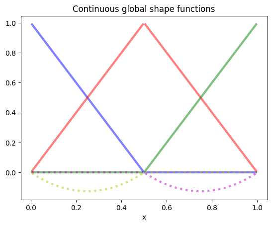
The global finite element space consists of functions of the form

\[ v(x) = \sum_i v_i \Theta_i(x) \]

where \(\Theta_i(x)\) are global shape functions. For the current example, we plotted them above. Note that when \(\Theta_i\) is restricted to a single element, we obtain either the zero function or a local shape function \(\theta_j\) of that element. A set of linear functionals \(G_j\) on the global finite element space having the property \(G_j(\Theta_j) = \delta_{ij}\) are called global degrees of freedom. Here \(\delta_{ij}\) denotes the Kronecker delta (equals 1 if \(i=j\) and 0 otherwise).

1.3. Coupling degrees of freedom

When some local degrees of freedom of distinct finite elements are fused together to form a single global degree of freedom, like we saw above, the result is called a coupling degree of freedom. In ngsolve, every global shape function, or equivalently every global degree of freedom, is given a CouplingType. When its CouplingType is LOCAL_DOF, it is not a coupling degree of freedom; all other values of CouplingType indicates a coupling degree of freedom.

for i in range(V.ndof):
    print(V.CouplingType(i))

COUPLING_TYPE.WIREBASKET_DOF
COUPLING_TYPE.WIREBASKET_DOF
COUPLING_TYPE.WIREBASKET_DOF
COUPLING_TYPE.LOCAL_DOF
COUPLING_TYPE.LOCAL_DOF

In this case, we see that all degrees of freedom are coupling degrees of freedom except the last two. Each degree of freedom marked LOCAL_DOF is identical to a local element degree of freedom within some element and its corresponding shape function is supported only on that single element. (You can verify that the last two shape functions in the current example are supported only on a single element by reviewing the plots of the global shape functions above.)

1.4. Approximation

One method of creating a finite element approximation of some given function \(f(x)\) is by the finite element interpolant. In ngsolve, another technique of creating approximations is offered as the default. This is in a method called Set that all GridFunctions have. It implements the Oswald approximation, obtained by first computing the \(L_2\) projection of \(f\) into each local finite element space and then assigning to every coupling degree of freedom the average of the degrees of freedom of the projection that were fused to form that coupling degree of freedom.

v.Set(sin(5*x))
plot1D(sin(5*x), mesh2, style=':b')
plot1D(v, mesh2, 'k')

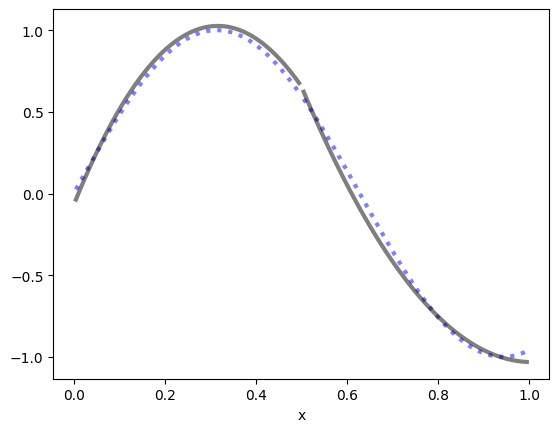
Clearly the approximation (solid curve) and the original (dotted sine curve) are close, but not identical.

Questions for discussion:

• What happens when you lower the degree on the same mesh?

• What happens when you increase the degree on the same mesh?

• How can you tell that these approximations are not obtained by the canonical finite element interpolation?

One way to improve the approximation is by increasing the degree. Another way is to make the mesh finer, as we see now.

1.5. The lowest order case

Partition the interval \([0, 1]\) using a uniform mesh \(\{ x_i = i h: i=0, \ldots, N \}\) of \(N+1\) points, where the mesh size is \(h = 1/N\) and set

\[ V_{h1} = \{ v: \; v \text{ is continuous and } v|_{[x_i, x_{i+1}]} \text { is linear }\}. \]

This vector space is called the lowest order Lagrange finite element space in the one-dimensional domain \([0,1]\). With \(N\) as a variable to adjust, let us make this space in ngsolve:

N = 5 
mesh = Make1DMesh(N) 
Vh1 = H1(mesh, order=1)
Vh1.ndof

6

From ndof outputs, we gather that the dimension of this space made using \(N\) elements appears to be equal to \(N+1\). Think about how to prove this.

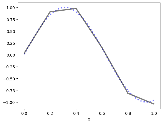
v = GridFunction(Vh1)
v.Set(sin(5*x))
plot1D(sin(5*x), mesh, style=':b')
plot1D(v, mesh, 'k')

Question for discussion

• Does the approximation appear to improve as \(h \to 0\) or \(N \to \infty\)?

for i in range(N+1):
    v.vec[:] = 0
    v.vec[i] = 1
    plot1D(v, mesh, style=colors[i], title='Global shape functions $\\Theta_i$')

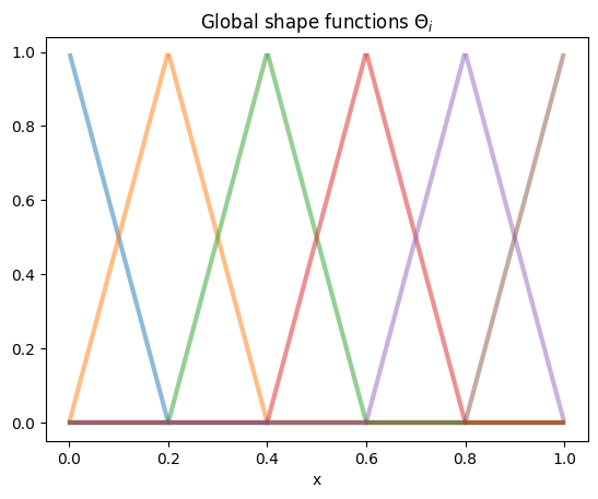
These functions \(\Theta_i \in V_{h1}\) with the property

\[ \Theta_i(x_j) = \delta_{ij} \]

at every mesh point \(x_j\) are often called hat functions colloquially. Note that although the statement \(\Theta_i(x_j) = \delta_{ij}\) only gives the values of \(\Theta_i\) at the mesh vertices \(x_j\), that is enough to determine the function \(\Theta_i\) everywhere, since it is linear in between the mesh points.

Questions for discussion

• Are \(\Theta_i\) linearly independent functions?

• What type of an object is sin(x) in the python code?

• Can you try other function expressions?

Please review NGSolve i-Tutorial 1.2 to learn more about CoefficientFunction objects.

1.6. Summary

We have seen

• the Lagrange and discontinuous Galerkin (DG) spaces in 1D,

• meshes of one-dimensional domains,

• evaluating finite element functions at points within an element,

• plotting 1D finite element functions using matplotlib,

• how functions in the spaces are captured by finite arrays,

• local degrees of freedom and coupling degrees of freedom,

• fusing local degrees of freedom to global ones,

• the Oswald approximation,

• global shape functions,

• type of mathematical expressions in ngsolve.